Phenomenology of axionic static neutron stars with masses in the mass-gap region

The current focus of theoretical astrophysicists, cosmologists, the theoretical particle physicists and astronomers lies in the sky, where current and future observations are anticipated and are expected to verify current theories or shake the ground in theoretical astrophysics and cosmology. The striking chorus of the new physics era observations initiated with the kilonova GW170817 event observation back in 2017 [1, 2]. This was a remarkable event exactly because a kilonova was involved in the observation. Thus astronomers of the LIGO-Virgo collaboration detected a gravitational wave and an electromagnetic wave emitted by the two neutron star (NS) merger. The two waves arrived almost simultaneously, since the electromagnetic wave arrived 1.74 s after the gravitational wave, and thus this event, almost instantly after the GW170817 announcement, casted serious doubts on the viability of theories of gravity that predict a gravitational wave speed different from that of light's, see for example [3–6], although theoretical refinements have been proposed for theories with stringy origin [7–9]. Many exciting events have been observed after the GW170817 event, with milestones being the GW190814 event [10] and the striking 2023 NANOGrav observation of a stochastic gravitational wave background, also confirmed by other pulsar timing array collaborations [11–14]. The former event captured the merging event of a black hole with a mysterious small mass object in the mass gap region $M\sim 2.6\,\mathrm{M}_{\odot}$, which could be the heaviest NS or the lightest black hole, but in both cases the outcome is exciting to say the least. To date nobody confirmed either of the aforementioned scenarios. Apparently the GW190814 event was a very valuable present offered by Nature to us, and can be the first event that gives us a hint for the existence of heavy NSs which cannot be explained by general relativity (GR) alone, even with the stiffest equation of state (EoS). What is needed to confirm the existence of such heavy NSs is either a NS merger event accompanied by a kilonova, or some observation of an low-spin isolated pulsar like the black-widow binary pulsar PSR J0952-0607 which has mass $M = 2.35\,\pm\,0.17$ [15] and it is quite close to the mass gap region. Motivated by this line of reasoning it stands to reason to think that GR itself might not suffice to describe heavy NSs in the mass gap region and that some modified gravity [16–20] can actually describe heavy NSs. This is a long-standing question in theoretical astrophysics and it is our personal belief that this question will be answered by a ground breaking near future kilonova NSs merger event. Thus NSs [21–25] are expected to be the test-bed of theories in the near future and for the next generations of scientists. There is a lot of physics involved in NSs and many theories can be experimentally tested, like for example nuclear physics theories with extreme matter conditions [26–37], high energy theoretical and particle physics theories [38–42], modified gravity descriptions of NSs, [43–52], see also [53–75] for the scalar-tensor approach and of course theoretical astrophysics scenarios, [76–90]. Motivated by the importance of the modified gravity perspective in NSs, in this work we shall examine static NSs in the context of an axionic scalar field theory. The axion is of profound theoretical importance and it is considered as an important dark matter candidate nowadays, and for a mainstream of important articles and reviews on axions see [91–110]. We shall consider several EoSs, using a phenomenological piecewise polytropic approach [111, 112], which is more appropriate for phenomenological reasons. With regard to the EoSs we shall consider the following, the SLy [113], the AP3-AP4 [114], the WFF1 [115], the ENG [116], the MPA1 [117], the MS1 and MS1b [118] and finally the APR EoS [119]. Among all these EoSs, the MPA1 seems to produce extremely viable NS phenomenology as it was shown in [74]. We tried the most important phenomenologically EoSs, which include stiff and mildly stiff EoSs, and the reason is that we wanted to check the variety of phenomenological implications. After our examination we found that some EoSs provide extreme maximum masses but these EoSs are excluded phenomenologically. Remarkably all the EoSs that provide viable results yield maximum NSs masses that respect the causal maximum mass of GR. Thus the inclusion of so many EoSs was from curiosity and for phenomenological completeness. We shall numerically solve the Einstein frame Tolman–Oppenheimer–Volkoff (TOV) equations and we shall calculate the Jordan frame Arnowitt–Deser–Misner (ADM) gravitational mass and radius of the NS [120]. The phenomenological viability of the NS will be tested by confronting the gravitational mass and radius data with all the current constraints on the masses and radii of NS. Specifically we shall consider three types of constraints which we call CSI, CSII and CSIII along with the latest NICER constraints. Specifically, the constraint CSI [76] constrains the radius of a $1.4\,\mathrm{M}_{\odot}$ mass NS to be $R_{1.4\,\mathrm{M}_{\odot}} = 12.42^{+0.52}_{-0.99}$ while that of an $2\,\mathrm{M}_{\odot}$ mass NS must be $R_{2\,\mathrm{M}_{\odot}} = 12.11^{+1.11}_{-1.23}\,$km. The constraint CSII [85] and constrains the radius of a $1.4\,\mathrm{M}_{\odot}$ mass NS to be $R_{1.4\,\mathrm{M}_{\odot}} = 12.33^{+0.76}_{-0.81}\,\mathrm{km}$, while CSIII [80] constrains the radius of an $1.6\,\mathrm{M}_{\odot}$ mass NS to be larger than $R_{1.6\,\mathrm{M}_{\odot}}\gt10.68^{+0.15}_{-0.04}\,$km, and also the radius corresponding to the maximum mass of the NS must be larger than $R_{M_{\mathrm{max}}}\gt9.6^{+0.14}_{-0.03}\,$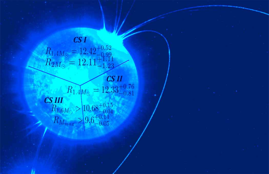km. We have gathered the constraints CSI, CSII and CSIII in figure 1. Regarding the NICER constraints, we shall consider two, which constrain the radius of an $M = 1.4\,\mathrm{M}_{\odot}$ mass NS to be $R_{1.4\,\mathrm{M}_{\odot}} = 11.34-13.23\,$km [121], which we call NICER I, while the second NICER constraint, to which we shall refer as NICER II, constraints again the radius of a $M = 1.4\,\mathrm{M}_{\odot}$ mass NS to be $R_{1.4\,\mathrm{M}_{\odot}} = 12.33-13.25\,$km. These are included in table 1. After presenting the phenomenological outcomes of our study we shall answer the theoretical question whether NS phenomenology originating by scalar-tensor inflationary potentials and axionic potentials NS produce similar results. The answer, to our surprise, lies in the affirmative. The surprise is due to the fact that although we use a natural inflation potential (axionic) the approximations used for this axion potential correspond to an era where the axion oscillates around the minimum of its potential and cosmologically redshifts as dark matter. We expected some differences, but the result is that the phenomenology of NSs is similar in the two cases. Now it is important to note that the axion potential in cosmological scales is basically a theory of gravity active at large scales, so the question is what is the relevance of this cosmological theory. The answer to this is that NSs are basically extreme gravitational environments, so in principle the large scale gravitational theory might have direct effects on such extreme gravity environments. Also we need to stress that the axionic NSs is composed by ordinary matter obeying one of the EoSs mentioned previously, but the gravitational equilibrium is controlled by the axionic scalar-tensor theory, thus it affects the maximum mass and the radius of the NS. Also note that we did not assume that actual dark matter particles, such as axions, exist inside the core of the NSs. This is a quite interesting perspective, but the exact treatment which somewhat change the theoretical framework used, since it would probably change the hydrodynamic equilibrium of the NS to some extent.

Zoom In Zoom Out Reset image size

Table 1. Viability Constraints for NS Phenomenology

Constraint	Mass and Radius
CSI	For $M = 1.4\,\mathrm{M}_{\odot}$, $R_{1.4\,\mathrm{M}_{\odot}} = 12.42^{+0.52}_{-0.99}$ and for $M = 2\,\mathrm{M}_{\odot}$, $R_{2\mathrm{M}_{\odot}} = 12.11^{+1.11}_{-1.23}\,$km.
CSII	For $M = 1.4\,\mathrm{M}_{\odot}$, $R_{1.4\,\mathrm{M}_{\odot}} = 12.33^{+0.76}_{-0.81}\,\mathrm{km}$.
CSIII	For $M = 1.6\,\mathrm{M}_{\odot}$, $R_{1.6\,\mathrm{M}_{\odot}}\gt10.68^{+0.15}_{-0.04}\,$km, and for $M = M_{\mathrm{max}}$, $R_{M_{\mathrm{max}}}\gt9.6^{+0.14}_{-0.03}\,$km.
NICER I	For $M = 1.4\,\mathrm{M}_{\odot}$, $11.34\,\mathrm{km}\lt R_{1.4\,\mathrm{M}_{\odot}}\lt13.23\,\mathrm{km}$
NICER II	For $M = 1.4\,\mathrm{M}_{\odot}$, $12.33\,\mathrm{km}\lt R_{1.4\,\mathrm{M}_{\odot}}\lt13.25\,\mathrm{km}$

Let us review in brief the formalism of scalar-tensor theories in the Einstein frame, and also extract the gravitational mass of NSs in the Einstein frame. We use the notation of [53] and we also shall work in Geometrized units ($G = c = 1$). The Jordan frame action of a non-minimally coupled scalar field is,

$$\begin{equation} \mathcal{S} = \int d^4x\frac{\sqrt{-g}}{16\pi}\left[\Omega\left(\phi\right)R-\frac{1}{2}g^{\mu \nu}\partial_{\mu}\phi\partial_{\nu}\phi-U\left(\phi\right)\right]+S_m\left(\psi_m,g_{\mu \nu}\right)\, , \end{equation} \tag{ 1 }$$

and upon conformally transforming this action, transformation,

$$\begin{equation} \tilde{g}_{\mu \nu} = A^{-2}g_{\mu \nu}\, ,\,\,\,A\left(\phi\right) = \Omega^{-1/2}\left(\phi\right)\, , \end{equation} \tag{ 2 }$$

we get the Einstein frame action,

$$\begin{equation} \mathcal{S} = \int d^4x\sqrt{-\tilde{g}}\left(\frac{\tilde{R}}{16\pi}-\frac{1}{2} \tilde{g}_{\mu \nu}\partial^{\mu}\varphi \partial^{\nu}\varphi-\frac{V\left(\varphi\right)}{16\pi}\right)+S_m\left(\psi_m,A^2\left(\varphi\right)\tilde{g}_{\mu \nu}\right)\, , \end{equation} \tag{ 3 }$$

with ϕ denoting the Einstein frame, which has a scalar potential $V(\varphi)$ related to the Jordan frame one $U(\phi)$ in the following way,

$$\begin{equation} V\left(\varphi\right) = \frac{U\left(\phi\right)}{\Omega^2}\, . \end{equation} \tag{ 4 }$$

Note that the passage from the Jordan to the Einstein frame is always possible in scalar-tensor theories, since a non-diverging conformal transformation can always be found. The passage from the Einstein-frame to the Jordan frame is not possible in higher derivative gravities that contain terms of the Gauss–Bonnet invariant, the Riemann and Ricci tensors. Furthermore, an important function is $\alpha(\varphi)$ which is defined as follows,

$$\begin{equation} \alpha\left(\varphi\right) = \frac{\mathrm{d} \ln A\left(\varphi\right)}{\mathrm{d} \varphi}\, , \end{equation} \tag{ 5 }$$

which is essential for the TOV equations and also $A(\varphi) = \Omega^{-1/2}(\phi)$. Since we consider static NSs, we shall consider a spherically symmetric metric,

$$\begin{equation} \mathrm{d}s^2 = -\mathrm{e}^{\nu\left(r\right)}\mathrm{d}t^2+\frac{\mathrm{d}r^2}{1-\frac{2 m\left(r\right)}{r}}+r^2\left(\mathrm{d}\theta^2+\sin^2\theta \mathrm{d}\phi^2\right)\, , \end{equation} \tag{ 6 }$$

with m(r) describing the gravitational mass of the NS, and r is the circumferential radius. The aim of the numerical solution we shall provide is the determination of the functions $\nu(r)$ and $\frac{1}{1-\frac{2 m(r)}{r}}$, which in the case of scalar-tensor gravity also receive contributions beyond the surface of the NSs, a feature absent in the GR case, and this is due to the fact that the scalar field affects these two metric functions beyond the surface of the star. Hence, there is no conventional matching of the spherically symmetric metric with the Schwarzschild metric at the surface of the star. This matching is performed at numerical infinity, where the effects of the scalar field have been smoothed away. Now by varying the Einstein frame action in the presence of ordinary matter, we get the TOV equations,

$$\begin{equation} \frac{\mathrm{d} m}{\mathrm{d}r} = 4\pi r^2 A^4\left(\varphi\right)\varepsilon+\frac{r}{2}\left(r-2m\left(r\right)\right)\omega^2+4\pi r^2V\left(\varphi\right)\, , \end{equation} \tag{ 7 }$$

$$\begin{equation} \frac{\mathrm{d}\nu}{\mathrm{d}r} = r\omega^2+\frac{2}{r\left(r-2m\left(r\right)\right)}\left[4\pi A^4\left(\varphi\right)r^3P-4\pi V\left(\varphi\right) r^3\right]+\frac{2m\left(r\right)}{r\left(r-2m\left(r\right)\right)}\, , \end{equation} \tag{ 8 }$$

$$\begin{align} \frac{d\omega}{\mathrm{d}r} & = \frac{4\pi r A^4\left(\varphi\right)}{r-2m\left(r\right)}\left(\alpha\left(\varphi\right)\left(\epsilon-3P\right)+ r\omega\left(\epsilon-P\right)\right)-\frac{2\omega \left(r-m\left(r\right)\right)}{r\left(r-2m\left(r\right)\right)}\nonumber\\ & \quad +\frac{8\pi \omega r^2 V\left(\varphi\right)+r\frac{\mathrm{d} V\left(\varphi\right)}{\mathrm{d} \varphi}}{r-2 m\left(r\right)}\, , \end{align} \tag{ 9 }$$

$$\begin{equation} \frac{\mathrm{d}P}{\mathrm{d}r} = -\left(\epsilon+P\right)\left[\frac{1}{2}\frac{\mathrm{d}\nu}{\mathrm{d}r}+\alpha \left(\varphi\right)\omega\right]\, , \end{equation} \tag{ 10 }$$

$$\begin{equation} \omega = \frac{\mathrm{d} \varphi}{\mathrm{d}r}\, , \end{equation} \tag{ 11 }$$

with $\alpha (\varphi)$ being defined in equation (5). For the numerical analysis we use the following initial conditions,

$$\begin{equation} P\left(0\right) = P_c\, ,\,\,\,m\left(0\right) = 0\, , \,\,\,\nu\left(0\right) = -\nu_c\, , \,\,\,\varphi\left(0\right) = \varphi_c\, ,\,\,\, \omega \left(0\right) = 0\, , \end{equation} \tag{ 12 }$$

with the initial values ν_c and ϕ_c being initially arbitrary, but the exact correct value will be obtained by performing a double shooting method, which aims to find the optimal values which render the scalar field at numerical infinity to be zero. Regarding the EoS for the nuclear matter, we shall use nine piecewise polytropic [111, 112] EoSs, and specifically, the SLy [113], the AP3-AP4 [114], the WFF1 [115], the ENG [116], the MPA1 [117], the MS1 and MS1b [118] and finally the APR EoS [119]. Let us now present the formula for the Einstein frame ADM mass of the NS, so we introduce the quantities $K_\mathrm{E}$ and $K_\mathrm{J}$ defined as follows,

$$\begin{equation} \mathcal{K}_\mathrm{E} = 1-\frac{2 m}{r_\mathrm{E}}\, , \end{equation} \tag{ 13 }$$

$$\begin{equation} \mathcal{K}_\mathrm{J} = 1-\frac{2 m_\mathrm{J}}{r_\mathrm{J}}\, , \end{equation} \tag{ 14 }$$

and are related as follows,

$$\begin{equation} \mathcal{K}_\mathrm{J} = A^{-2}\mathcal{K}_\mathrm{E}\, . \end{equation} \tag{ 15 }$$

Accordingly, the Jordan and Einstein frame radii are related as follows,

$$\begin{equation} r_\mathrm{J} = A r_\mathrm{E}\, , \end{equation} \tag{ 16 }$$

and accordingly the Jordan frame ADM gravitational mass is,

$$\begin{equation} M_\mathrm{J} = \lim_{r\to \infty}\frac{r_\mathrm{J}}{2}\left(1-\mathcal{K}_\mathrm{J} \right) \, , \end{equation} \tag{ 17 }$$

while the Einstein frame ADM gravitational mass is,

$$\begin{equation} M_\mathrm{E} = \lim_{r\to \infty}\frac{r_\mathrm{E}}{2}\left(1-\mathcal{K}_\mathrm{E} \right) \, . \end{equation} \tag{ 18 }$$

Asymptotically equation (15) yields,

$$\begin{equation} \mathcal{K}_\mathrm{J}\left(r_\mathrm{E}\right) = \left(1+\alpha\left(\varphi\left(r_\mathrm{E}\right)\right)\frac{\mathrm{d} \varphi}{\mathrm{d} r}r_\mathrm{E} \right)^2\mathcal{K}_E\left(\varphi\left(r_E\right)\right)\, , \end{equation} \tag{ 19 }$$

with $r_\mathrm{E}$ denoting the Einstein frame radius at numerical infinity and also $\frac{\mathrm{d}\varphi }{\mathrm{d}r} = \frac{\mathrm{d}\varphi }{\mathrm{d}r}\Big{|}_{r = r_\mathrm{E}}$. Combining equations (13)–(19) we get the formula for the Jordan frame ADM gravitational mass of the NS,

$$\begin{equation} M_\mathrm{J} = A\left(\varphi\left(r_\mathrm{E}\right)\right)\left(M_\mathrm{E}-\frac{r_\mathrm{E}^{2}}{2}\alpha \left(\varphi\left(r_\mathrm{E}\right)\right)\frac{\mathrm{d}\varphi }{\mathrm{d}r}\left(2+\alpha\left(\varphi\left(r_\mathrm{E}\right)\right)r_E\frac{\mathrm{d} \varphi}{\mathrm{d}r} \right)\left(1-\frac{2 M_\mathrm{E}}{r_\mathrm{E}} \right) \right)\, , \end{equation} \tag{ 20 }$$

and recall that $\frac{\mathrm{d}\varphi }{\mathrm{d}r} = \frac{\mathrm{d}\varphi }{\mathrm{d}r}\Big{|}_{r = r_\mathrm{E}}$. Also the radius of the NS in the Jordan frame denoted as R is related to the Einstein frame one R_s as follows,

$$\begin{equation} R = A\left(\varphi\left(R_s\right)\right)\, R_s\, , \end{equation} \tag{ 21 }$$

and note that the Einstein frame mass is determined at the surface of the star where $P(R_s) = 0$. Our aim with the numerical analysis is to calculate the Einstein frame mass and radii of the NS and from these to calculate their Jordan frame counterparts and construct the M − R graphs of the NSs.

2.1. Axion NSs

Now let us consider the axionic scalar-tensor theory which we shall assume that governs the Universe at cosmological and astrophysical scales. The axionic theory is basically a dark matter theory. Let us consider the general form of such theory in a cosmological context, and then we specify the theory for the NS study we aim to perform in this work. In the context of the misalignment axion [94, 96], the axion possesses a primordial U(1) Peccei–Quinn symmetry which is basically broken during the inflationary era. The misalignment axion commences its evolution towards the minimum of its scalar potential which has the following form,

$$\begin{equation} V_a\left(\phi \right) = m_a^2\,f\,_a^2\left(1-\cos \left(\frac{\phi}{f_a}\right) \right)\, , \end{equation} \tag{ 22 }$$

where initially its initial value φ_i at the time it commences its motion towards the bottom of its potential is $\phi_i\sim f_a$, with f_a being the axion decay constant, which is of the order $f_a\gt10^{9}\,$GeV. During its motion towards the minimum of the potential the axion satisfies, $\phi/f_a\lt1$, thus for the original axionic theory, the scalar potential can be approximated by,

$$\begin{equation} V_a\left(\phi \right)\simeq \frac{1}{2}m_a^2\phi^2\, , \end{equation} \tag{ 23 }$$

an approximation which is valid when $\phi\lt f_a$ and this covers the eras in which the axion moves towards the minimum of the scalar potential. After the axion reaches the minimum it commences coherent oscillations, approximately when the Hubble rate of the Universe H is of the order as the axion mass m_a , so basically when $H\sim m_a$. Note that this occurred primordially, since the present day Hubble rate is $H\sim 10^{-33}\,$eV so it is too small to be compared to the axion mass, which in most cases, the axion mass is in he range $m_a\sim 10^{-10}-10^{-24}\,$eV. After this era primordial era with $H\sim m_a$, the axion oscillates and its energy density redshifts as cold dark matter and the axion basically becomes a non-thermal dark matter candidate. For the purposes of this work, we shall consider the non-minimally coupled Jordan frame axionic theory developed in [122], in which the Jordan frame potential of equation (1) in Geometrized units reads,

$$\begin{equation} U\left(\phi\right) = \Lambda^4\left(1-\cos\left(\frac{\phi}{f_a} \right) \right)\, , \end{equation} \tag{ 24 }$$

while the non-minimal coupling function $\Omega(\phi)$ in equation (1) reads,

$$\begin{equation} \Omega\left(\phi\right) = 1+\xi \phi^n\, . \end{equation} \tag{ 25 }$$

The parameter n can take values $n = 2,4,{\ldots}$ so we focus here to n = 2. The parameter ξ shall be assumed to take large values $\xi\sim 10^4\gg 1$. Then we get,

$$\begin{equation} \frac{\mathrm{d} \varphi }{\mathrm{d} \phi} = \sqrt{\frac{1}{4\pi}}\sqrt{\frac{12\xi^2\phi^2+1\xi\phi^2}{4\left(1+\xi\phi^2\right)^2}}\, , \end{equation} \tag{ 26 }$$

so assuming that in the interior of the star, the following approximation holds true,

$$\begin{equation} \xi^2\phi^2\gg \xi \phi^2\gg 1\, . \end{equation} \tag{ 27 }$$

Equation (26) becomes,

$$\begin{equation} \frac{\mathrm{d} \varphi }{\mathrm{d} \phi} = \sqrt{\frac{3}{4\pi}}\frac{\xi \phi}{1+\xi\phi^2}\, , \end{equation} \tag{ 28 }$$

so upon integration of the above we get,

$$\begin{equation} \varphi = \frac{\sqrt{3}}{2\sqrt{4\pi}}\ln \left(1+\xi \phi^2\right)\, , \end{equation} \tag{ 29 }$$

or equivalently,

$$\begin{equation} 1+\xi \phi^2 = \mathrm{e}^{2\sqrt{\frac{4\pi}{3}}\varphi}\, . \end{equation} \tag{ 30 }$$

The conformal factor $A(\phi)$ expressed in terms of the Einstein frame scalar field ϕ reads,

$$\begin{equation} A\left(\varphi\right) = \mathrm{e}^{-\sqrt{\frac{4\pi}{3}}\varphi}\, , \end{equation} \tag{ 31 }$$

and the function $\alpha(\varphi)$ which is defined in equation (5) takes the following form,

$$\begin{equation} a\left(\varphi\right) = \alpha = -\sqrt{\frac{4\pi}{3}}\, . \end{equation} \tag{ 32 }$$

Finally, since we are interested in an era in which $\phi/f_a\ll 1$, the Einstein frame potential takes the following form,

$$\begin{equation} V\left(\varphi\right) = -\frac{\Lambda^4}{2f_a\xi}\left(1-\mathrm{e}^{-\alpha \varphi} \right)\mathrm{e}^{-2\alpha\varphi}\, , \end{equation} \tag{ 33 }$$

where we expanded the cosine term in the Jordan frame in the limit $\phi/f_a\ll 1$. Now regarding the free parameters, the axion mass determines the axion mass so in natural units it must be $\Lambda^4/f_a^2\sim m_a^2$ so in order to have an axion with mass $m_a\sim 10^{-10}\,$eV with $f_a\sim 10^9\,$GeV we have $\Lambda\sim 10^4\,$eV. Also $\xi\gt-\left(\frac{M_p}{f_a\pi}\right)^2$ where M_p is the reduced Planck mass in natural units. In Geometrized units the parameter ξ must be $\xi\sim 10^4$. In the end of the calculations, the approximation (27) must be checked if it holds true in the center and at the surface of the star.

2.2. Results and confrontation with the data

In this section we shall present the outcomes of our numerical analysis. We used a rigorous double shooting LSODA python-based integration method which is variant of the pyTOV-STT code developed in [123]. The double shooting technique is aimed for finding the optimal initial conditions for ν_c and ϕ_c defined in equation (12) that make the values of the scalar field at numerical infinity near zero. With our numerical analysis we extracted the Einstein frame radii and gravitational masses for the NSs, using all the nine different EoSs, and we found the Jordan frame quantities using the formulas of the previous sections. Using the Jordan frame gravitational masses and radii we constructed the M − R graphs for all the EoSs we mentioned earlier. We also took account the constraints CSI, CSII and CSIII, which are pictorially represented in figure 1. Recall that constraint CSI [76] indicates that a NS with mass $1.4\,\mathrm{M}_{\odot}$ must have radius $R_{1.4\,\mathrm{M}_{\odot}} = 12.42^{+0.52}_{-0.99}$, while for the case of a $2\,\mathrm{M}_{\odot}$ mass NS the radius must be $R_{2\mathrm{M}_{\odot}} = 12.11^{+1.11}_{-1.23}\,$km. Considering the constraint CSII [85], for an $1.4\,\mathrm{M}_{\odot}$ mass NS, the radius must be $R_{1.4\,\mathrm{M}_{\odot}} = 12.33^{+0.76}_{-0.81}\,\mathrm{km}$. Finally, considering the CSIII constraint, regarding NSs with masses $1.6\,\mathrm{M}_{\odot}$, the radius must be $R_{1.6\,\mathrm{M}_{\odot}}\gt10.68^{+0.15}_{-0.04}\,$km and also for the maximum mass of a NS, the radius must be $R_{M_{\mathrm{max}}}\gt9.6^{+0.14}_{-0.03}\,$km. In all the M − R graphs we considered, we also included the NICER I constraint regarding $M = 1.4\,\mathrm{M}_{\odot}$ mass NSs with 90% credibility [121] and indicates that $R_{1.4\,\mathrm{M}_{\odot}} = 11.34-13.23\,$km regarding $M = 1.4\,\mathrm{M}_{\odot}$ mass NSs. Also a refinement of the NICER constraint was given in the literature [87] which takes into account the heavy black-widow binary pulsar PSR J0952-0607 which has mass $M = 2.35\pm 0.17$ [15]. We shall call this NICER II in the M − R plots. 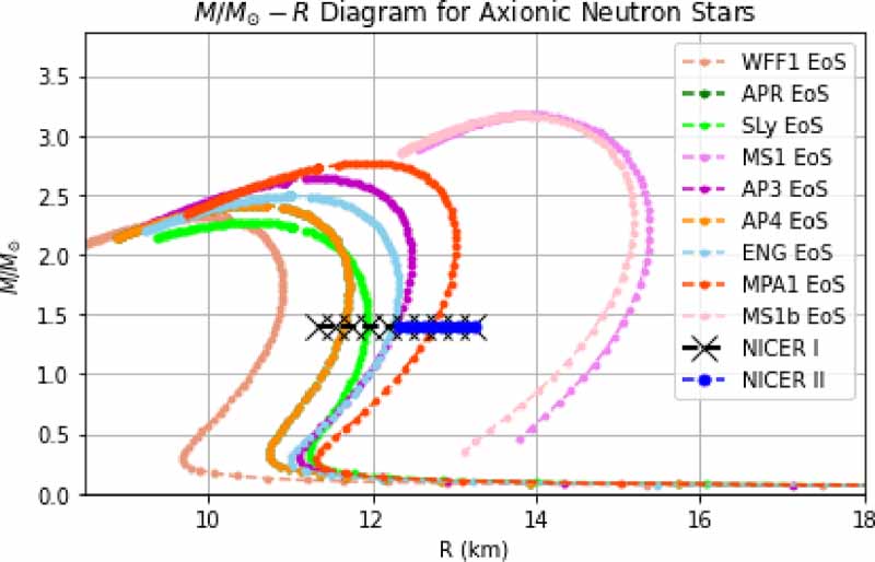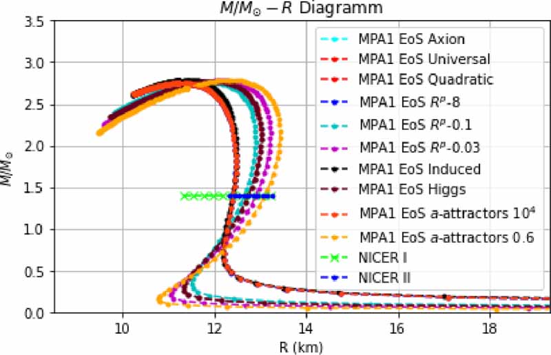The NICER II indicates that the radius of a $M = 1.4\,\mathrm{M}_{\odot}$ NS has to be $R_{1.4\,\mathrm{M}_{\odot}} = 12.33-13.25\,$km. For reading and referral convenience, we present the NICER I and NICER II constraints and constraints on the tidal deformability from the GW170817 merger [1] in table 9. In figure 2 we present the M − R graphs for the axionic NSs, regarding the Jordan frame masses and radii, considering the following EoSs WFF1, SLy, APR, MS1, AP3, AP4, ENG, MPA1, MS1b and we confront the M − R graphs with the constraints NICER I [121] and NICER II [87] (see table 2). From figure 2 it is abundantly clear that three EoSs pass the final test regarding axionic NSs, the ENG (marginally pass), the AP3 (marginally pass too) and the MPA1, which is the most optimal EoS. Now this is quite intriguing, since in [74], which described a different context and perspective, the MPA1 EoS was also found to be at the most optimal EoS phenomenologically. Specifically in [74] the scalar-tensor theories studied, were basically inflationary attractors. In this work however we consider an axionic scalar-tensor theory in which the axion is considered to be in the oscillating era regime of its potential. In simple words, the inflationary attractors describe viable inflationary theories while in the present context, the axion describes a dark matter theory, at least when the axion oscillations commence and the potential is approximately a quadratic one. Thus remarkably, two classes of conceptually different scalar-tensor theories overlap for the MPA1 EoS. This is quite intriguing and it is tempting to compare the inflationary attractors with the axionic theory for the MPA1 EoS, which seems to enjoy an elevated role among all the EoSs we considered. The comparison is made in figure 3. As it can be seen, the M − R graph for the inflationary attractors and for the axionic scalar-tensor theories are quite similar and in fact the axionic scalar-tensor theory along with the Induced inflation and the Higgs inflation cases, are well confronted with the NICER I and II constraints, all the three enjoying an elevated position compared to the other models. Using the extracted data of our numerical analysis for the Jordan frame masses and radii for the NSs, we also confronted these with the CSI, CSII and CSIII constraints. We gathered the results in several tables in the text for reading convenience. In table 3 we present the maximum masses of NSs that belong to the mass-gap region, for the corresponding EoSs that achieve this. Also in tables 4 and 5 we confront the NSs radii with the CSI constraint, when NSs with masses $M\sim 2M_{\odot}$ are considered. Also in tables 6 and 7 we confront the NSs radii with the CSI constraint, for NSs with masses $M\sim 1.4\,\mathrm{M}_{\odot}$. Furthermore, in tables 8 and 9 we confront the NSs radii with the CSII constraint, when NSs with masses $M\sim 1.4\,\mathrm{M}_{\odot}$ are considered. Also in tables 10 and 11 we confront the radii of NSs with masses $M\sim 1.6\,\mathrm{M}_{\odot}$ with the constraint CSIII and also in tables 12 and 13 we confront again the radii of NSs with maximum masses, with the constraint CSIII. Regarding the maximum masses, there exist several models that predict a maximum mass inside the mass-gap region for the axionic NSs but only the AP3 and the MPA1 and marginally the ENG EoS predict a NS with mass in the mass-gap region. More importantly, for these viable cases, the maximum mass is well below the causal 3 solar masses limit of GR. Recall that the causal mass GR limit for static NSs is also respected for modified gravity theories too [44], and for GR it is [125, 126],

$$\begin{equation} M_{\mathrm{max}}^{CL} = 3\,\mathrm{M}_{\odot}\sqrt{\frac{5\times 10^{14}\,\mathrm{g\,cm}^{-3}}{\rho_u}}\, , \end{equation} \tag{ 34 }$$

Zoom In Zoom Out Reset image size

Zoom In Zoom Out Reset image size

Table 2. NICER I AND NICER II Constraints for the radius of a $M = 1.4\,\mathrm{M}_{\odot}$ NS and Constraints for the Tidal Deformability from GW170817

NICER I	$11.34\,\mathrm{km}\lt R_{1.4\,\mathrm{M}_{\odot}}\lt13.23\,\mathrm{km}$ [121]
NICER II	$12.33\,\mathrm{km}\lt R_{1.4\,\mathrm{M}_{\odot}}\lt13.25\,\mathrm{km}$ [87]
GW170817	$\tilde{\Lambda} \unicode{x2A7D} 800$ [1]
GW170817	$\Lambda(1.4\,\mathrm{M}_{\odot}) \unicode{x2A7D} 800$ [1]
GW170817	$\tilde{\Lambda} = 245^{+453}_{-151}$ [124]

Table 3. Maximum Masses for Axionic NSs in the Mass Gap Region.

Model	MPA1 EoS	MS1b EoS	AP3 EoS	MS1 EoS
$M_{\mathrm{MAX}}$	$M_{\mathrm{MPA1}} = 2.771\,\mathrm{M}_{\odot}$	$M_{\mathrm{MS1b}} = 3.167\, \mathrm{M}_{\odot}$	$M_{\mathrm{AP3}} = 2.638\,\mathrm{M}_{\odot}$	$M_{\mathrm{MS1}} = 3.175\,\mathrm{M}_{\odot}$

Table 4. Axionic NSs vs CSI for NS Masses $M\sim 2\,\mathrm{M}_{\odot}$, $R_{2M_{\odot}} = 12.11^{+1.11}_{-1.23}\,$km, for the SLy, APR, WFF1, MS1 and AP3 EoSs. The 'x' denotes non-viability.

Model	SLy EoS	APR EoS	WFF1 EoS	MS1 EoS	AP3 EoS
Axionic NSs Radii	$R_{\mathrm{SLy}} = 11.675\,$Km	$R_{\mathrm{APR}} = 11.650\,$Km	$R_{\mathrm{WFF1}} = x$	$R_{\mathrm{MS1}} = x$	$R_{\mathrm{AP3}} = 12.467\,$Km

Table 5. Axionic NSs vs CSI for NS Masses $M\sim 2\,\mathrm{M}_{\odot}$, $R_{2\,\mathrm{M}_{\odot}} = 12.11^{+1.11}_{-1.23}\,$km, for the AP4, ENG, MPA1 and MS1b. The 'x' denotes non-viability.

Model	AP4 EoS	ENG EoS	MPA1 EoS	MS1b EoS
Axionic NSs	$R_{\mathrm{AP4}} = 11.650\,$Km	$R_{\mathrm{ENG}} = 12.263\,$Km	$R_{\mathrm{MPA1}} = 13.014\,$Km	$R_{\mathrm{MS1b}} = x$

Table 6. Axionic NSs vs CSI for NS Masses $M\sim 1.4\,\mathrm{M}_{\odot}$, $R_{1.4\,\mathrm{M}_{\odot}} = 12.42^{+0.52}_{-0.99}$, for the SLy, APR, WFF1, MS1 and AP3 EoSs. The 'x' denotes non-viability.

Model	SLy EoS	APR EoS	WFF1 EoS	MS1 EoS	AP3 EoS
Axionic NSs Radii	$R_{\mathrm{SLy}} = 11.934\,$Km	$R_{\mathrm{APR}} = 11.645\,$Km	$R_{\mathrm{WFF1}} = x$	$R_{\mathrm{MS1}} = x$	$R_{\mathrm{AP3}} = 12.333$

Table 7. Axionic NSs vs CSI for NS Masses $M\sim 1.4\,\mathrm{M}_{\odot}$, $R_{1.4\,\mathrm{M}_{\odot}} = 12.42^{+0.52}_{-0.99}$, for the AP4, ENG, MPA1 and MS1b. The 'x' denotes non-viability.

Model	AP4 EoS	ENG EoS	MPA1 EoS	MS1b EoS
Axionic NSs Radii	$R_{\mathrm{AP4}} = 11.645\,$Km	$R_{\mathrm{ENG}} = 12.236\,$Km	$R_{\mathrm{MPA1}} = 12.74\,$Km	$R_{\mathrm{MS1b}} = x$

Table 8. Axionic NSs Radii vs CSII for NS Masses $M\sim 1.4\,\mathrm{M}_{\odot}$, $R_{1.4\,\mathrm{M}_{\odot}} = 12.33^{+0.76}_{-0.81}\,\mathrm{km}$, for the SLy, APR, WFF1, MS1 and AP3 EoSs. The 'x' denotes non-viability.

Model	SLy EoS	APR EoS	WFF1 EoS	MS1 EoS	AP3 EoS
Axionic NSs Radii	$R_{\mathrm{SLy}} = 11.934\,$Km	$R_{\mathrm{APR}} = 11.645\,$Km	$R_{\mathrm{WFF1}} = x$	$R_{\mathrm{MS1}} = x$	$R_{\mathrm{AP3}} = 12.287\,$Km

Table 9. Axionic NSs vs CSII for NS Masses $M\sim 1.4\,\mathrm{M}_{\odot}$, $R_{1.4\,\mathrm{M}_{\odot}} = 12.33^{+0.76}_{-0.81}\,\mathrm{km}$, for the AP4, ENG, MPA1 and MS1b. The 'x' denotes non-viability.

Model	AP4 EoS	ENG EoS	MPA1 EoS	MS1b EoS
Axionic NSs Radii	$R_{\mathrm{AP4}} = 11.645\,$Km	$R_{\mathrm{ENG}} = 12.236\,$Km	$R_{\mathrm{MPA1}} = 12.748\,$Km	$R_{\mathrm{MS1b}} = x$

Table 10. Axionic NSs vs CSIII for NS Masses $M\sim 1.6\,\mathrm{M}_{\odot}$, $R_{1.6\,\mathrm{M}_{\odot}}\gt10.68^{+0.15}_{-0.04}\,$km, for the SLy, APR, WFF1, MS1 and AP3 EoSs. The 'x' denotes non-viability.

Model	SLy EoS	APR EoS	WFF1EoS	MS1 EoS	AP3 EoS
Axionic NSs Radii	$R_{\mathrm{SLy}} = 11.924\,$Km	$R_{\mathrm{APR}} = 11.705\,$Km	$R_{\mathrm{WFF1}} = 10.892\,$Km	$R_{\mathrm{MS1}} = x$	$R_{\mathrm{AP3}} = x$

Table 11. Axionic NSs vs CSIII for NS Masses $M\sim 1.6\,\mathrm{M}_{\odot}$, $R_{1.6\,\mathrm{M}_{\odot}}\gt10.68^{+0.15}_{-0.04}\,$km, for the AP4, ENG, MPA1 and MS1b. The 'x' denotes non-viability.

Model	AP4 EoS	ENG EoS	MPA1 EoS	MS1b EoS
Axionic NSs Radii	$R_{\mathrm{AP4}} = 11.705\,$Km	$R_{\mathrm{ENG}} = 12.308\,$Km	$R_{\mathrm{MPA1}} = 12.871\,$Km	$R_{\mathrm{MS1b}} = 14.902\,$Km

Table 12. Axionic NSs Maximum Masses and the Corresponding Radii vs CSIII, $R_{M_{\mathrm{max}}}\gt9.6^{+0.14}_{-0.03}\,$km, for the SLy, APR, WFF1, MS1 and AP3 EoSs. The 'x' denotes non-viability.

Model	APR EoS	SLy EoS	WFF1 EoS	MS1 EoS	AP3 EoS
Axionic NSs $M_{\mathrm{max}}$	$M_{\mathrm{APR}} = 2.417\,\mathrm{M}_{\odot}$	$M_{\mathrm{SLy}} = 2.272\,\mathrm{M}_{\odot}$	$M_{\mathrm{WFF1}} = 2.320\,\mathrm{M}_{\odot}$	$M_{\mathrm{MS1}} = 3.175\,\mathrm{M}_{\odot}$	$M_{\mathrm{AP3}} = 2.638\,\mathrm{M}_{\odot}$
Axionic NSs Radii	$R_{\mathrm{APR}} = 10.579\,$Km	$R_{\mathrm{SLy}} = 10.567\,$Km	$R_{\mathrm{WFF1}} = 9.911\,$Km	$R_{\mathrm{MS1}} = 13.910\,$Km	$R_{\mathrm{AP3}} = 11.359\,$Km

Table 13. Axionic NSs Maximum Masses and the and the correspondent vs CSIII, $R_{M_{\mathrm{max}}}\gt9.6^{+0.14}_{-0.03}\,$km, for the AP4, ENG, MPA1 and MS1b. The 'x' denotes non-viability.

Model	AP4 EoS	ENG EoS	MPA1 EoS	MS1b EoS
Axionic NSs $M_{\mathrm{max}}$	$M_{\mathrm{AP4}} = 2.417\,\mathrm{M}_{\odot}$	$M_{\mathrm{ENG}} = 2.492\,\mathrm{M}_{\odot}$	$M_{\mathrm{MPA1}} = 2.771\,\mathrm{M}_{\odot}$	$M_{\mathrm{MS1b}} = 3.167\,\mathrm{M}_{\odot}$
Axionic NSs Radii	$R_{\mathrm{AP4}} = 10.579\,$Km	$R_{\mathrm{ENG}} = 11.011\,$Km	$R_{\mathrm{MPA1}} = 11.944\,$Km	$R_{\mathrm{MS1b}} = 13.838\,$Km

where ρ_u stands for the reference density used to separate the causal region and the low-density region, up to which the overall EoS is known and the corresponding pressure is $P_u(\rho_u)$. The causal EoS is,

$$\begin{equation} P_{sn}\left(\rho\right) = P_{u}\left(\rho_u\right)+\left(\rho-\rho_u\right)c^2\, , \end{equation} \tag{ 35 }$$

and for rotating NSs, the causal limit is,

$$\begin{equation} M^{CL,rot}_{\mathrm{max}} = 3.89\,\mathrm{M}_{\odot}\sqrt{\frac{5\times 10^{14}\,\mathrm{g\,cm}^{-3}}{\rho_u}}\, , \end{equation} \tag{ 36 }$$

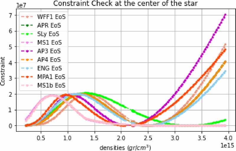
but this does not concern us in this work, we quote it only for completeness. Now regarding the confrontation of the axionic NSs with the constraints CSI and CSII, three EoSs are entirely excluded, the WFF1, the MS1 and the MS1b EoSs. While in the case of the constraint CSIII, the WFF1 is entirely incompatible with it. Finally, we need to check the validity of the approximation (27) for the center and the NS surface. This is presented in figures 4 and 5 respectively. As it can be seen, the constraint is well satisfied both at the center and the surface of the NS.

Zoom In Zoom Out Reset image size

Zoom In Zoom Out Reset image size

In this work we considered the effects of an axionic scalar-tensor theory on static NSs. Specifically, we considered the axionic theory in the regime that the axion field oscillates around the minimum of its scalar potential and cosmologically redshifts as cold dark matter. Thus this scalar-tensor theory is somewhat distinct from inflationary scalar-tensor theories. We presented the essential features of the axion scalar-tensor theory and demonstrated how this theory is basically a dark matter theory in which the axion starts to behave as cold dark matter post-inflationary. Specifically, when the Hubble rate of the Universe becomes of the same order as the axion mass, the axion begins coherent oscillations around the minimum of its potential and redshifts as cold dark matter. The scalar-tensor theory we chose to describe the axion basically takes into account the fact that the axion oscillates around the potential minimum, so we took into account this approximation in order to appropriately describe the potential in this regime. We constructed the TOV equations for this axionic theory, and we specified the initial conditions at the center of the star. The we used a double shooting method in order to find the optimal initial conditions at the center of the star, for the scalar field value and the metric function, which make the scalar field to smooth out to zero at the numerical infinity. From our numerical analysis we calculated the Einstein frame gravitational mass and radii for the NSs and accordingly we found their Jordan frame counterparts using the formulas we provided for the ADM mass and Jordan frame radius. The numerical calculation was performed for nine distinct and physically motivated EoSs, the WFF1, the SLy, the APR, the MS1, the AP3, the AP4, the ENG, the MPA1 and the MS1b, using the piecewise polytropic description for each EoS. From the resulting data we constructed the M − R graphs (Jordan frame quantities) and finally we confronted the resulting NS phenomenology with the mainstream of NS constraints available in the literature. Specifically we used the NICER constraint and also a variant form of it [87], which we called NICER II, based on heavy black-widow binary pulsar PSR J0952-0607 with mass $M = 2.35\pm 0.17$ [15], which constraints the radius of an $M = 1.4\,\mathrm{M}_{\odot}$ mass NS to have a radius $R_{1.4\,\mathrm{M}_{\odot}} = 12.33-13.25\,$km. Also we used three extra well-known constraints which we named CSI, CSII and CSIII appearing in table 1. The resulting phenomenology was deemed quite interesting for various reasons. Firstly, all the viable EoSs for the axionic stars, predict a maximum mass in the mass-gap region with $M_{\mathrm{max}}\gt2.5\,\mathrm{M}_{\odot}$, however with the maximum mass being lower than the 3 solar masses causal EoS limit. The three EoSs which are compatible with all the constraints we imposed are the AP3, ENG and the MPA1, with the latter enjoying an elevated role among all EoS. In fact the MPA1 EoS produces the most well-fitted results which are compatible with all the constraints. Also, the WFF1, MS1 and MS1b EoSs, are entirely excluded from describing viable static NSs. Our results are similar with the ones obtained when inflationary attractors NSs are considered, and this intriguing fact made us compare the axionic NSs with the inflationary attractors. As we demonstrated the resulting M − R graphs are quite similar, thus although the two scalar-tensor theories have a different context, with the axionic one corresponding to a dark matter theory (and its approximations), the two theories produce quite similar NS phenomenology. In conclusion, the MPA1 EoS is deemed phenomenologically important, and it produces NSs with maximum masses inside the mass gap region, below the 3 solar masses limit though. Thus this EoS along with the scalar-tensor axionic model and the inflationary attractor models will constitute a class of models which can explain any future observation of NS with mass in the mass-gap region but below 3 solar masses.

Finally, an important comment is in order, which must be explored in a deeper way. Specifically, the NICER's results and constraints are derived using ray tracing within the framework of GR, but the external metrics of NSs in scalar-tensor gravity differ from those in GR. Strictly speaking, employing results from NICER or GW170817 can be problematic. This issue, is very important from a phenomenological point of view, and it was addressed in [127–129]. We hope to discuss this issue further in the future, in the context of inflationary and axionic scalar-tensor theories of gravity.

This research has been is funded by the Committee of Science of the Ministry of Education and Science of the Republic of Kazakhstan (Grant No. AP14869238).

No new data are created. The data that support the findings of this study are available upon reasonable request from the authors.