


Abstract
In situ measurements of coronal mass ejections (CMEs) when they pass over an interplanetary probe are one of the main ways we directly measure their properties. However, such in situ profiles are subject to several observational constraints that are still poorly understood. This work aims at quantifying one of them, namely, the aging effect, using a CME simulated with a three-dimensional magnetohydrodynamical code. The synthetic in situ profile and the instantaneous profile of the magnetic field strength differ more from each other when taken close to the Sun than far from it. Moreover, out of three properties we compute in this study (i.e., size, distortion parameter, and expansion speed), only the expansion speed shows a dependence of the aging as a function of distance. It is also the property that is the most impacted by the aging effect as it can amount to more than 100 km s−1 for CMEs observed closer than 0.15 au. This work calls for caution when deducing the expansion speed from CME profiles when they still are that close to the Sun since the aging effect can significantly impact the derived properties.
Export citation and abstract BibTeX RIS

Original content from this work may be used under the terms of the Creative Commons Attribution 4.0 licence. Any further distribution of this work must maintain attribution to the author(s) and the title of the work, journal citation and DOI.
1. Introduction
In situ measurements constitute one of the main ways to study the evolution of coronal mass ejections (CMEs) while they propagate in interplanetary space. However, such measurements are subject to many constraints. For instance, it has been shown recently that the profiles of the magnetic field components of the same CME probed by two different spacecraft separated by even just a few degrees can show strong discrepancies (Winslow et al. 2022; Lugaz et al. 2023; Regnault et al. 2023b). This is consistent with the finding presented by Lugaz et al. (2018) where the coherence scale of the magnetic field components amounted to about ≲15°. In addition, the effect of evolution of the CME during the time it takes to pass over the spacecraft (referred to as the "aging effect") has been shown to significantly impact the properties we infer from parameter profiles measured by the spacecraft at 1 au (Osherovich et al. 1993; Démoulin et al. 2020; Regnault et al. 2023a).
There have been efforts to study CMEs using in situ data from multiple spacecraft at different heliocentric distances (e.g., Leitner et al. 2007; Good et al. 2019; Davies et al. 2020; Lugaz et al. 2020; Salman et al. 2020; Zhuang et al. 2023). These studies are either case studies or are limited to magnetic field measurements, as one of the spacecraft is often on a planetary mission without plasma measurements. However, multispacecraft studies of CMEs allow us to partially overcome some observational constraints without making strong assumptions about the CME structure (force-free state, or the presence of an invariant axis) that cannot be thoroughly verified.
Another way to overcome these strong observational constraints is through numerical simulations. In particular, they allow us to produce synthetic profiles and compare them with instantaneous profiles (corresponding to a 1D cut through the structure at a given time) and to do so at different heliocentric distances. This particular application allows us, then, to quantify the aging effect at different heliocentric distances.
Understanding the aging effect becomes more and more important since the recent launch of the Parker Solar Probe (PSP; Fox et al. 2016; Raouafi et al. 2023). We have started to measure CMEs when they are very close to the Sun (<0.1 au; see, e.g., Long et al. 2023; McComas et al. 2023; Romeo et al. 2023), and to this day, it is still unclear how strong the aging effect is closer to the Sun. The aging effect close to the Sun could be much greater than at 1 au, and thus, data analysis following procedures developed for in situ measurements at 1 au to obtain CME properties (e.g., size, expansion) could be flawed. Besides, going back to in situ measurements, understanding the CME global magnetic configuration based on limited measurements can be attempted using CME flux rope (FR) models, but the aging effect can bring large uncertainties in that case as well.
This paper aims at studying a simulated 3D magnetohydrodynamic (MHD) FR to quantify the aging effect at different distances from the Sun. More precisely, we compare synthetic data profiles and instantaneous profiles of a simulated CME. The substantial advantage of simulations is that for all time steps, all the data are available everywhere in the simulation domain. It thus provides a very convenient method to be able to perform such a study. Simulations have been used to compare simulated and derived properties of CMEs from remote observations (e.g., see Lugaz 2005), the forces acting on CMEs (e.g., see Shen et al. 2014), the fitted versus true CME magnetic morphology (e.g., see Riley et al. 2004; Al-Haddad et al. 2011), and the evolution of the CME size (Al-Haddad et al. 2019) but not, to the best of our knowledge, to investigate the aging effect.
In this work, we refer to "temporal profile" as the profile corresponding to the synthetic in situ data at a given spacecraft location (similar to real in situ measurements) and "spatial profile" as the instantaneous 1D cut at a given time. This is illustrated in Figure 1 where φ is the physical parameter we measure where the red dashed line shows the spatial profile and the black arrow is where the data for the temporal profile is obtained. Note that here we consider a fixed position for sake of simplicity, which is a safe assumption at 1 au. However, closer to the Sun, the spacecraft motion could induce even more differences between the temporal and spatial profiles.
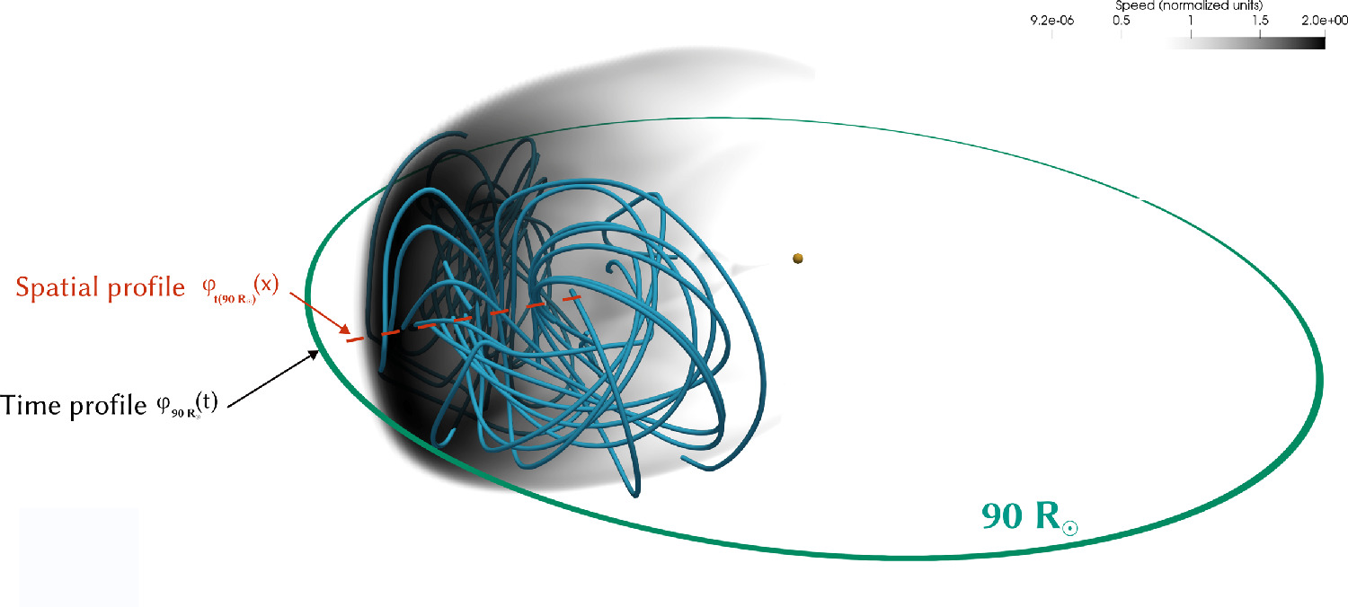
Figure 1. Three-dimensional visualization when the CME reaches 90 R⊙. The gray color map encodes the magnitude of the speed in the meridional plane. Blue lines are the magnetic field lines plotted from a radial line starting at 57 R⊙ and ending at 78 R⊙. The yellow sphere corresponds to the position of the Sun, with a radius of 1 R⊙. The green circle corresponds to 90 R⊙.
Download figure:
Standard image High-resolution imageWe use the same distinction between temporal and spatial to describe the parameters inferred from these profiles, namely the distortion parameter (DiP; Nieves-Chinchilla et al. 2018), the radial expansion speed, and the radial size. The difference between the temporal and spatial profiles is related to the evolution of the CME properties as it passes over the spacecraft, and as such this study investigates the aging effect. The rest of the Letter is organized as follows. In Section 2, we describe the simulation and the methodology to derive temporal and spatial profiles. In Section 3, the results of the analysis are presented, and we conclude in Section 4.
2. Methodology
In this section, we summarize the simulation that is used for this study. More details can be found in Regnault et al. (2023c).
2.1. Three-dimensional MHD Simulation of a CME
We use the PLUTO code to solve the 3D MHD equations in an adaptive mesh refinement (AMR; Mignone et al. 2012) spherical grid (r, θ, ϕ) from the low corona (1 R⊙) up to 2 au. The AMR grid allows us to keep a high spatial resolution exclusively around the propagating FR. The solar wind is initialized with a polytropic Parker solar wind solution. The magnetic field configuration of the Sun is a dipole mimicking that of the Sun during its quiet phase. The solution is then evolved in time with an ideal equation of state. The solar wind is driven by heating produced by setting the ratio of specific heats γ to 1.05. This leads to an almost isothermal corona at about 106 K.
To model the initial magnetic structure of the CME, we use the modified Titov–Démoulin FR model (Titov et al. 2014). It allows an analytical formulation of an FR magnetic structure anchored at the Sun. We initialize the FR out of equilibrium, and it thus erupts quickly after its insertion. In Regnault et al. (2023c), the propagation of six different initial magnetic FRs was investigated for different values of the FR thickness and the initial magnetic field strength. For this study, we use the thin2 FR from Regnault et al. (2023c). We chose a thin FR because it does not have an issue with a fast stream behind the FR, while the thick FRs do.
Out of the three thin FRs, we do not choose thin3 since this FR has a very large propagation speed at 1 au (FR front speed >1000 km s−1). This might not be representative of a typical CME. Furthermore, we chose thin2 over thin1 because thin1 has a propagation speed at 1 au, which is almost equal to the solar wind speed in its wake (see Figure 8 in Regnault et al. 2023c). Thus, it indicates that the overtaking solar wind plasma might have interacted with the FR during its propagation and also brings uncertainties in the following estimations.
Once the FR has erupted, we follow its position by using the axial magnetic field (see Regnault et al. 2023c for more details). The CME is propagating radially. Our study starts when the FR reaches 30 R⊙ (≈0.15 au) to ensure that we have enough points in time for the synthetic profile and ends when the FR reaches 210 R⊙ (≈1 au). All the profiles shown in this study are made in "ideal" conditions, i.e., at the nose of the radially propagating CME in the plane where the FR is located.
2.2. Defining the CME Boundaries
Figure 2 shows the comparison of the temporal and spatial profiles for the magnetic and plasma parameters when the CME is at 110 R⊙. For spatial profiles, we use the data when the CME center (see below for details) is detected to be at 110 R⊙. The magnetic field components in this figure are expressed in the RTN coordinates where the R, T, and N each correspond to the r, φ, and θ of the simulation. To find the CME position, we use its axial magnetic field (BN) on which we perform a Gaussian fit. The center position of the Gaussian then determines the position of the CME (for more details, see Regnault et al. 2023c).
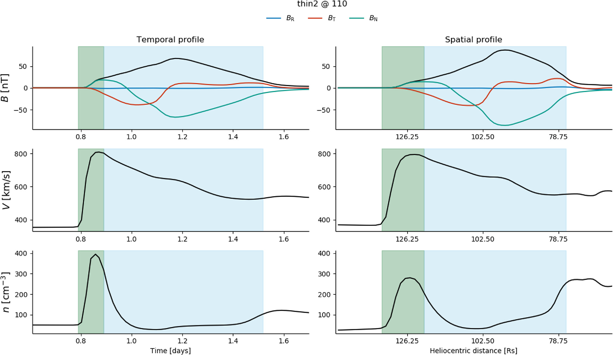
Figure 2. Synthetic temporal profile (left) and spatial profile of the simulated CME in RTN coordinates. The green and blue areas correspond to the sheath and the ME, respectively. From top to bottom, we show the magnetic field strength and its components in nT, the speed in kilometers per second, and the density in cubic centimeters inverse.
Download figure:
Standard image High-resolution imageThe green and blue shaded areas in Figure 2 show the simulated sheath region and the magnetic ejecta (ME), respectively. The latter corresponds to the magnetic structure being expelled from the solar corona, and the sheath corresponds to the compressed solar wind in front of the ME when it is fast enough to drive a shock. We describe below how we define the start and end times of both regions. This figure shows that, while the magnetic field strength profile (black curve) is rather symmetric in the synthetic temporal profile (left), it appears asymmetric with more magnetic flux at the end of the ME spatial profile (right). This highlights already that the aging effect can have a significant impact on the CME properties deduced from single-point in situ profiles. In Section 3, we quantify these differences.
We use the increase of the speed and density for the beginning of the sheath. The maximum of Bθ is used for the start of the FR (start of the smooth rotation of the Bθ component due to the presence of the FR). Unlike the beginning of the sheath or of the FR, there are no clear signatures to use for the end of the FR. We thus decide to define the end of the FR when the magnetic field strength goes under 20% of the maximum magnetic field. Then, we apply these criteria to define the CME boundaries for every CME location between 30 and 210 R⊙ with a step of 10 R⊙.
3. Assessment of the Aging Effect
3.1. Difference between the Spatial and Temporal Profiles as a Function of Distance
Figure 3 shows on the left a direct comparison of the normalized temporal and spatial profiles at four different distances from the Sun. These profiles are normalized by subtracting the average value of the magnetic field strength profile and dividing by its standard deviation. Such a protocol allows us to compare directly the shape of the profiles at different distances without being affected by differences in their magnitude. The right panel shows the evolution of the absolute average difference between the spatial and temporal profiles. This is calculated as the sum of the difference (Δ profile) of each profile divided by the number of points of the profile, and this is done for each pair of profiles from 30 to 210 R⊙.

Figure 3. Left panels: comparison of the temporal and spatial profiles when the CME is at 50, 100, 150 and 200 R⊙. These profiles are normalized; see main text for more details. The right panel shows the difference between the temporal and spatial profiles as a function of distance. Details are in Section 3.1.
Download figure:
Standard image High-resolution imageThe left panels show that, at all distances, when the CME is still close to the Sun, most of the profile discrepancies occur at the front of the CME. The peak of the magnetic field is also slightly shifted toward the front for the temporal profile and is not centered as for the spatial profile. This difference could be due to the fact that the spatial profile actually probes the CME magnetic field when its back is comparatively closer to the Sun. When the CME position is at 50 R⊙, its back is at 31.9 R⊙. However, by the time that the back arrives at 50 R⊙ (where the temporal profile is measured), it has had time to expand and thus for the magnetic field strength to decrease.
It is interesting to note that, farther away from the Sun, for instance at 150 or 200 R⊙ (third and fourth panels on the left), we do not observe such differences at the front. It then means that while the CME expands during its propagation, it does not expand enough to cause a strong discrepancy between the time and spatial profiles.
The right panel of Figure 3 shows that the difference between the spatial and temporal profile decreases as a function of distance from a 0.7 difference at 0.15 au to a 0.3 difference at 1 au. These results then suggest that the aging effect (i.e., difference between the spatial and the temporal profile) is more predominant close to the Sun.
3.2. Influence of the Aging Effect on the Inferred CME Properties
In the previous section, we highlighted the effect of aging on the in situ profile by comparing directly the value of spatial and temporal profiles of the magnetic field. In this section, we quantify the aging effect by comparing the CME properties we derive from the temporal and spatial profiles at different heliocentric distances.
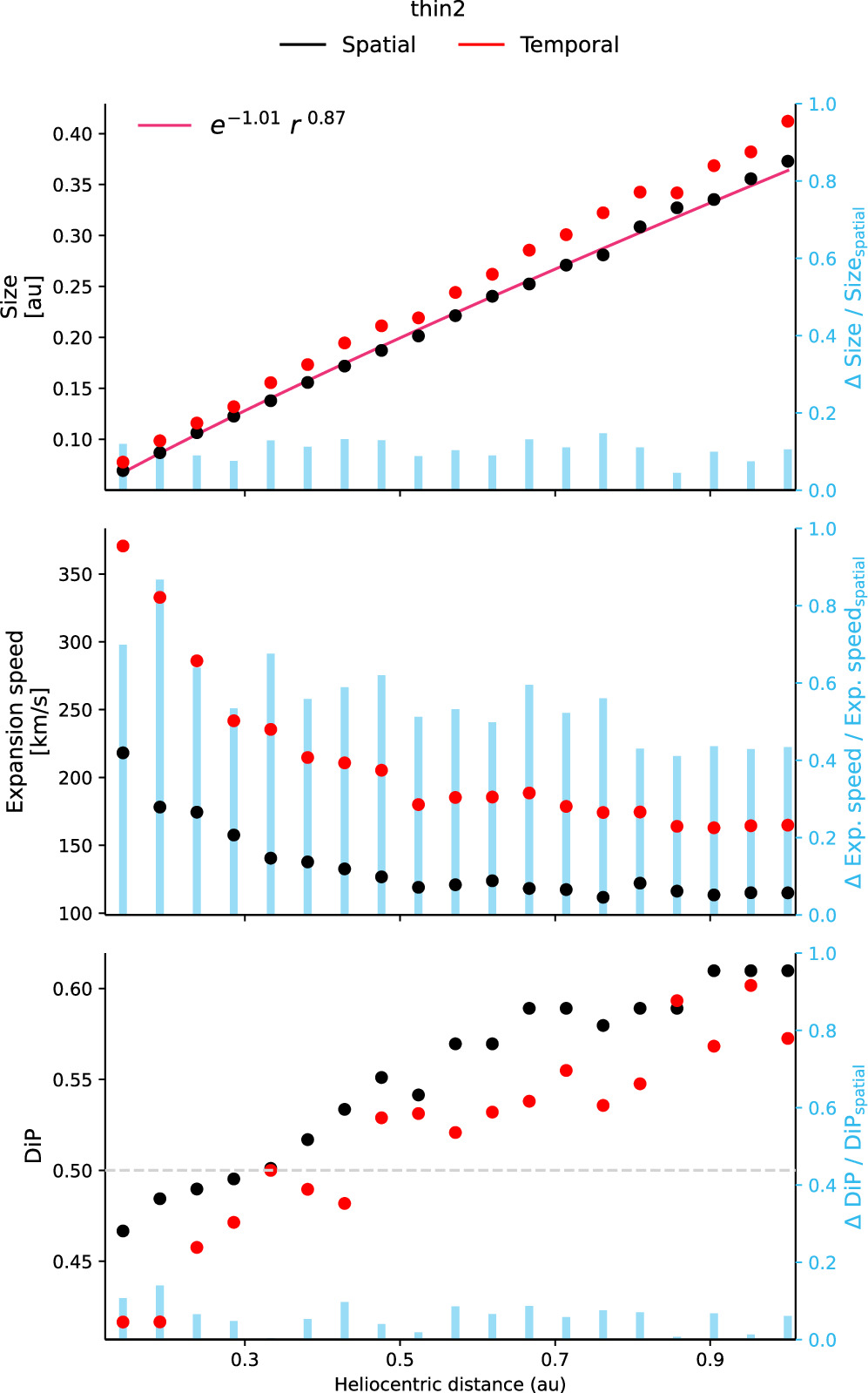
Figure 4 shows the DiP of the ME profile, which is a quantification of the asymmetry of the magnetic field strength profile (see Nieves-Chinchilla et al. 2018 for more details), the expansion speed in kilometers per second, and the size of the CME in astronomical units deduced from the temporal profile (in red) and from the spatial profile (in black). The blue histogram shows the absolute difference between the parameters deduced from both profiles relative to the parameter deduced from the spatial profile.
Figure 4. Comparison of the CME properties deduced from the temporal profile (in red) and from the spatial profile (in black). From top to bottom, we show the size of the CME in astronomical units, the expansion speed in kilometers per second, and the DiP. All the parameters are a function of heliocentric distance. In the first panel, the purple curve corresponds to a power-law fit. Blue bars show the absolute difference between the parameter deduced from the temporal and spatial profiles relative to the parameter deduced with the spatial profile. For sake of comparison, all the y-axes are set to the same scale.
Download figure:
Standard image High-resolution image
3.2.1. Size of the CME
The temporal size (in red) shown in the first panel of Figure 4 is computed by multiplying the average speed within the ME region and the ME duration. We find that, as expected, the CME size increases as a function of distance. We fit a power law to it and find a power-law index of 0.87 (purple curve). As a matter of comparison, Al-Haddad et al. (2019) studied the size evolution of a simulated "writhed" and "twisted" magnetic structure up to 0.6 au. They find that the size of the writhed structure evolves as a function of distance with a power-law index of 0.705 and the twisted structure with a power-law index of 0.661. From observations, we typically find a power-law index of 0.61–0.92 (see Scolini et al. 2021; Zhuang et al. 2023, and references therein), while on the higher end, the evolution of the simulated CME follows well what has been found in these aforementioned studies.
Considering the relative difference between the sizes (blue histograms), there is no clear trend as a function of distance. On average, there is an overestimation of the "true" size (i.e., the spatial size) of about 10% when using the temporal profile to compute it. This is very likely due to the fact that when computing the size, we average the speed, which is an overestimation of the actual speed. This also highlights that the size is changing as the CME passes over the spacecraft.
3.2.2. Expansion Speed
The second panel of Figure 4 shows the expansion speed, which is computed using the same formula for both profiles:
with Vfront and Vrear the speed at the front and at the rear of the temporal and spatial profiles when performing a fit to these profiles. This suggests that all the speed variation in the ME comes from its expansion and thus that it does not decelerate significantly (see discussion in Regnault et al. 2023b). In this section, we can now actually verify this assumption.
First, we observe that the expansion speed derived from the temporal profile decreases from 360 to 170 km s−1 from 0.14 to 1 au. The spatial expansion speed decreases from 220 to 110 km s−1. At 1 au, we measure an average expansion speed of about 30–50 km s−1 for solar cycles 23 and 24 (Gopalswamy et al. 2015). However, Figure 10 of Richardson & Cane (2010) shows that an expansion speed of 100–200 km s−1 is measured in CMEs at 1 au. The somewhat high expansion speed found here of the simulated CME is also in agreement with the power-law index for the size, which is high but still within the typical observational range.
The relative difference between the spatial and temporal expansion speeds decreases as a function of heliospheric distance. It is about 70% close to the Sun and 40% around 1 au. This result suggests that using in situ data below typically 0.5 au tends to overestimate the actual expansion speed of the CME at a given time by a significant amount. It means that, for instance, at 0.3 au (distance of Solar Orbiter from the Sun when it is at its closest), the bias due to the aging effect may cause an overestimation of the speed of 90 km s−1. Below 0.15 au, distances at which PSP has already probed some CMEs, the difference can be as high as 150 km s−1.
3.2.3. DiP
The third panel of Figure 4 shows the DiP as a function of the heliocentric distance for the spatial and temporal profiles. It shows where half of the total magnetic flux is reached within the ME (Nieves-Chinchilla et al. 2018). It is used to quantify the asymmetry of a parameter profile; if DiP = 0.5 (dashed gray line in the first panel of Figure 4) the profile is symmetric.
We observe that, when the CME propagates, the magnetic field profile is first compressed toward the front until 0.3 au and then is compressed toward the back of the ME. From 0.15 to 1 au, the DiP increases and reaches a plateau around 0.57 for the temporal and around 0.62 for the spatial DiP. We find that using in situ data, we tend to always underestimate the DiP by 0.03 (average absolute difference) wherever the CME is measured. We do not observe any clear trend at different distances.
4. Discussion and Conclusions
In this work, we use a 3D MHD simulation of a propagating CME to directly compare the spatial and temporal profiles of a CME between 0.15 and 1 au and the properties we deduce from them. Such comparisons allow us to quantify the aging effect, which is an effect that is still poorly constrained and extremely difficult to quantify relying only on single-spacecraft data, and still very difficult in the rare occurrence of a multispacecraft CME (Regnault et al. 2023a). Even in simulations such as this one, quantifying the aging effect is not a straightforward matter. Indeed, for this study, we only compared profiles that were measured at the nose of the CME front. This location was chosen because this is where the aging is expected to be larger due to the greater speed. Moreover, if the probe were few degrees away from the nose, then it would also cut toward the axial direction of the FR. Thus, spatial changes of the FR might come at play and make the study of the aging effect more difficult.
While the simulation was performed under ideal MHD assumptions (no explicit viscosity or resistivity), we observe that the temporal profiles are actually smoother than the actual in situ ones. This is due to the numerical dissipation induced by the spatial discretization of the simulation domain. In order to assess the effect of nonideal terms on the aging effect, simulations at higher resolution would be needed, which are out of the scope of this study.
We find that the aging effect impacts all the parameters discussed in this Letter, namely, the expansion speed, the size, and the DiP of the CME, to an amount of 55, 11, and 6% respectively averaged over the heliocentric distance. The expansion speed is the parameter that is the most impacted by the aging effect. However, the dependence on heliocentric distance is not the same for all the parameters. From Section 3.1, we expect a greater aging effect close to the Sun than far from it. Only the expansion speed shows a decrease of the magnitude of the aging effect as a function of distance; no clear trend is observed for the size and the DiP. In others words, the greater the expansion speed, the greater the aging effect, but only for the expansion speed. We would have expected to observe this trend also in the size of the CME, but it is not the case. It then means that no matter how big the CME, the aging effect should be about the same.
The CME studied in this work expands at a rate that is on the high end of the observational range, which explains its long duration at 1 au. This means that the results presented here could constitute an upper bound to the aging effect. It would be very interesting to replicate this study by comparing with other simulations or extend it by studying other parameters to confirm or refute our findings.
Acknowledgments
F.R., N.A., and W.Y. acknowledge grants 80NSSC21K0463 and AGS1954983. F.R. and N.A. acknowledge grant 80NSSC22K0349. N.L. and F.R. acknowledge grant 80NSSC20K0700. B.Z. acknowledges grants 80NSSC23K1057 and AGS2301382. C.J.F. acknowledges support from the Wind grant 80NSSC19K1293.