2.1 LULC-related parameters

In this study, the MODIS MCD12Q1 version 6 (Friedl and Sulla-Menashe, 2019) was employed to ascertain the plant functional types (PFT) as well as other non-vegetative land categories at a spatial resolution of 1 km spanning the years 2001 to 2020. The integrity of the MODIS land cover product has been established through a 10-fold cross-validation accuracy assessment using the Terrestrial Ecosystem Parameterization database (Sulla-Menashe et al., 2019). This land cover product offers richer and more flexible land cover data with higher accuracy and substantially less year-to-year stochastic variation in classification results (Sulla-Menashe et al., 2019). Being the sole operational global land cover product available with annual intervals, it addresses a significant gap in the realm of global change research.

The original MODIS land cover data were first resampled to 1 km from its original 500 m resolution using a majority resampling method in GEE. At such a high 1 km resolution, we did not consider the proportion of different land cover types within each grid. Instead, we assigned 100 % of a grid cell to the major land cover type. Specifically, the MCD12Q1 LC_Type 5 PFT classification layer was used to determine the distributions of the seven PFTs, as well as lake, urban, and glacier, following the method outlined in Ke et al. (2012) and summarized below:

• The seven PFTs include needleleaf evergreen trees, needleleaf deciduous trees, broadleaf evergreen trees, broadleaf deciduous trees, shrub, grass, and crop. These PFTs were further reclassified into 15 categories (Table S1 in the Supplement) that are typically used in LSMs based on the rules presented in Bonan et al. (2002a) with the assistance of 1 km precipitation and surface air temperature from WorldClim V1 (Hijmans et al., 2005).

• Grass was reclassified as C₃ and C₄ grass using the approach presented by Still et al. (2003), with the assistance of monthly LAI (processed in Sect. 2.2.1) and meteorological variables from WorldClim V1.

• The “non-vegetated land” was classified as the barren soil class.

• The “permanent snow and ice” was assigned as the glacier land unit.

• Global lakes were identified based on the classification of “water bodies” over the global land, constrained using the global land mask obtained from Natural Earth (https://www.naturalearthdata.com/, last access: 6 June 2023).

• The urban land unit was determined based on the MODIS “urban and built-up” classification. These urban grids were further classified into three urban classes, namely, tall building district (TBD), high density (HD), and medium density (MD), based on Jackson et al. (2010; hereinafter referred to as J2010). J2010 generated global urban extent maps for the TBD, HD, and MD classes at a spatial resolution of 1 km, based on rules of building height and vegetation coverage fraction (https://gdex.ucar.edu/dataset/188a_oleson/file.html, last access: 6 June 2023). However, the J2010 dataset is temporally static and cannot reflect changes in urban boundaries over time. Therefore, we reclassified the yearly MODIS urban land class as TBD, HD, and MD based on the J2010 dataset using the nearest-neighbor sampling method for each year.

After determining the distribution of 15 PFTs, bare soil, lake, glacier, and urban land, any remaining 1 km grids were assigned as ocean (Table S1). It should be noted that the wetland land unit was not explicitly classified in this study. This is because, instead of treating wetlands as an individual land unit, many LSMs (e.g., ELM2 and CLM5) integrate wetland functioning processes prognostically within other land units where a surface water storage component is implemented to represent wetland functioning.

2.2 Vegetation-related parameters

2.3 Soil-related parameters

We obtained the SoilGrids 2.0 data with an original resolution of 250 m (Poggio et al., 2021) to prepare soil properties. SoilGrids 2.0 is generated using machine learning based on multiple data sources of soil profiles and remote sensing data (Hengl et al., 2017). The soil product underwent rigorous quantitative evaluation using a cross-validation method, which ensures alignment with established pedo-landscape features and provides spatial uncertainty to guide product users (Poggio et al., 2021). SoilGrids 2.0 provides percent clay, percent sand, and soil organic matter for six standard soil layers: 0–5, 5–15, 15–30, 30–60, 60–100, and 100–200 cm. The original SoilGrids 2.0 data obtained from GEE were processed at 1 km resolution with multiple layers using an area-weighted averaging method. To facilitate the demonstration, we restructured the six soil layers vertically into ELM2's 10 effective soil layers (0–1.8, 1.8–4.5, 4.5–9.1, 9.1–16.6, 16.6–28.9, 28.9–49.3, 49.3–82.9, 82.9–138.3, 138.3–229.6, and 229.6–380.2 cm) using the nearest-neighbor method. It should be noted that the lake module in ELM2 and CLM5 requires soil properties, but the SoilGrids 2.0 data may not provide coverage over water surfaces. To address this, we utilized the nearest-neighbor sampling method to map the 1 km soil properties onto the terrestrial water surface.

2.4 Topography-related parameters

We employed the digital elevation from the Multi-Error-Removed Improved-Terrain DEM (MERIT DEM; Yamazaki et al., 2019) to obtain topography-related parameters. The MERIT DEM provides globally consistent elevation data at 90 m resolution, distinguished by its exceptional vertical accuracy. This accuracy was rigorously validated against ICESat's lowest elevations in both forested and non-forested regions and was further benchmarked using the UK's premium airborne lidar DEM (Yamazaki et al., 2019). We first acquired the 1 km elevation and standard deviation of elevation using GEE based on the original 90 m elevation. Further, we calculated the slope, aspect, sky view factor, and terrain configuration factor from the 1 km elevation using the parallel computing tool developed by Dozier (2022). The sky view factor represents the proportion of visible sky limited by adjacent terrain, and the terrain configuration factor describes the proportion of adjacent terrain which is visible to the ground target. Finally, to drive the parameterization of subgrid topographical effects on solar radiation (Hao et al., 2022) in ELM2, we calculated the sin (slope)⋅sin (aspect) and sin (slope)⋅cos (aspect) for calculating the local solar incident angle, as well as two normalized angle-related factors, the sky view factor, and terrain configuration factor by cos (slope). It is important to note that the standard deviation of elevation calculated in this study is specific to the 1 km resolution simulation. For applications requiring coarser resolutions (e.g., 0.5°), the standard deviation should be recalculated directly from the 1 km elevation rather than averaging from the 1 km standard deviation of elevation.

2.5 Comparison between new and existing land surface parameters

In this study, since the data sources used to develop the 1 km global land surface parameters have already undergone rigorous validation, we do not perform additional evaluations against reference datasets (e.g., observations). Instead, our focus is on comparing the newly developed 1 km parameters with those from K2012 and the ELM2/CLM5 default parameters. The K2012 parameters were obtained through personal communication (refer to the “Data availability” section for details). The ELM2/CLM5 default parameters were sourced from the Community Earth System Model (CESM) input data repository (https://svn-ccsm-inputdata.cgd.ucar.edu/trunk/inputdata/, last access: 6 June 2023). Given the different resolutions of these datasets (our new parameters at 1 km, K2012 at 0.05°, and the ELM2/CLM5 defaults with varying resolutions), we adapt our comparison at different resolutions for different variables.

For PFT parameters, we aggregated both the 1 km new parameters and the 0.05° K2012 data to the 0.5° resolution of the ELM2/CLM5 default. For non-vegetated land units (i.e., urban, glacier, and lake), we upscaled the 1 km new parameters to a 0.05° resolution to align with the ELM2/CLM5 default. It is important to note that the urban parameter in K2012 is only available for the Northern Hemisphere, due to limitations in data acquisition.

When comparing LAI, we aggregated the 1 km new and K2012 LAI to 0.5° resolution, matching the ELM2/CLM5 default LAI/SAI resolution. We excluded the comparison of SAI from our analysis due to the limited availability of the global K2012 dataset, from which we only acquired coverage for North America. We have not included a comparison of vegetation canopy height (top and bottom parameters) in our study. This is because the K2012 dataset does not contain these parameters, and the ELM2/CLM5 default parameters in the CESM input data repository provide only tabular values for each PFT rather than spatially variable canopy heights for tree PFTs.

For soil and topography-related parameters, our comparison was limited to the 1 km new parameters and the ELM2/CLM5 default, as K2012 does not include these parameters. Specifically, for soil comparisons, we aggregated the new 1 km parameters to 0.083° resolution to match the ELM2/CLM5 default soil parameters. For topography, given that the ELM2/CLM5 default parameters is a combination of 1 km and 10 arcmin data sources, we simplify the comparison by aggregating both the new 1 km parameters and ELM2/CLM5 default to 0.5° resolution, including elevation and slope.

3.1 Experiment design

To demonstrate the capability of 1 km datasets, we conducted ELM2 simulations over CONUS at the resolution of 1 km, using the newly developed 1 km land surface parameters for 2010. We used atmospheric forcing from the Global Soil Wetness Project Phase 3 (GSWP3; Kim, 2017) with a spatial resolution of 0.5° to drive ELM. The spatial homogeneity of atmospheric forcings within 0.5° grid cells guarantees that the spatial variability of the ELM-simulated variables (e.g., latent heat) within 0.5° grid cells is solely attributable to the heterogeneity of the 1 km land surface parameters. There are approximately 12 million effective grids over CONUS. We ran ELM for 5 years (2010–2014), and the last year's simulation was used for analysis. We specifically analyzed the annual mean of surface layer soil moisture (SM, m³ m⁻³), latent heat (LH, W m⁻²), emitted longwave radiation (ELR, W m⁻²), and absorbed shortwave radiation (ASR, W m⁻²).

3.2 Spatial scaling analysis

We conducted a spatial scaling analysis following the method described in Vergopolan et al. (2022) on the 1 km ELM simulation data to better understand how k-scale spatial heterogeneity in the four ELM-simulated variables (mentioned in Sect. 3.1) induced only by spatial heterogeneity of land surface parameters changes across spatial scales. First, we performed upscaling by averaging the 1 km ($\mathrm{1}/\mathrm{120}$°) land surface parameters and the four ELM-simulated variables to coarser spatial scales, i.e., λ_scale of $\mathrm{1}/\mathrm{60}$, $\mathrm{1}/\mathrm{40}$, $\mathrm{1}/\mathrm{30}$, $\mathrm{1}/\mathrm{24}$, $\mathrm{1}/\mathrm{20}$, and $\mathrm{1}/\mathrm{10}$°, and we calculated the spatial standard deviation (σ_scale) within each 0.5°×0.5° box at each spatial scale (Table 2). Second, we quantified the changes in spatial variability at different spatial scales compared to the original 1 km resolution by calculating the ratio of σ_scale to σ_1 km. Third, we fitted a $\log \left(\frac{{\mathit{\sigma }}_{\mathrm{scale}}}{{\mathit{\sigma }}_{\mathrm{1}\mathrm{km}}}\right)\propto \mathit{\beta }\times \log \left(\frac{{\mathit{\lambda }}_{\mathrm{scale}}}{{\mathit{\lambda }}_{\mathrm{1}\mathrm{km}}}\right)$ relationship, where β is an indicator to quantify data spatial variability persistence across scales (Hu et al., 1997). A more negative β indicates a larger dependency of data spatial variability on spatial scales, resulting in a higher information loss, denoted as ${\mathit{\gamma }}_{\mathrm{scale}}=(\mathrm{1}-{\mathit{\sigma }}_{\mathrm{scale}}/{\mathit{\sigma }}_{\mathrm{1}\mathrm{km}})\times \mathrm{100}$ %. In this study, we focus on information loss at a 12 km scale, denoted as γ_12 km. For simplicity in the subsequent discussion, γ_12 km will be referred to as γ in the results section. Given the possibility that β may not demonstrate significant temporal variation (Mälicke et al., 2020) and considering that our scaling analysis is intended for demonstration purposes, our spatial scaling analysis is based on the annual mean of ELM2 simulations.

Table 2Spatial resolution and pixel number at different spatial scales.

Download Print Version | Download XLSX

It is crucial to clarify that the upscaled 1 km simulation results in the spatial scaling analysis are not equivalent to the results obtained from a coarse-resolution ELM conducted using upscaled parameters. The spatial scaling analysis is intended to emphasize the value of high-resolution modeling in capturing fine-scale spatial variabilities and to highlight the contributions of high-resolution land surface parameters on the simulated variables.

3.3 Attribution analysis utilizing XML methods

We conducted additional analysis to determine the primary land surface parameters that influence the spatial scaling of ELM simulations. We employed XML methods, specifically the eXtreme Gradient Boosting (XGBoost; Chen and Guestrin, 2016) machine learning (ML) algorithm and the game theoretic approach SHapley Additive exPlanations (SHAP; Lundberg and Lee, 2017; Lundberg et al., 2018, 2020). XML methods were utilized to assess the influence of land surface parameters on the spatial variability and information loss of ELM2 simulations across CONUS. Taking spatial variability as an example, we first computed the standard deviation (σ) within each 0.5°×0.5° grid for both 1 km resolution land surface parameters and simulations. Then, we train a machine learning model to predict the spatial variability of each simulated variable (i.e., SM, LH, ELR, ASR). We used the spatial variability (i.e., σ) and mean (μ) of the land surface parameters and μ of precipitation and temperature as predictor variables, and we use the simulated variable's σ as the target variable. After training the machine learning model, we used SHAP to quantify the relative importance and determine which factors were most important in driving the spatial variability of the simulations. Similarly, we used this approach to identify the most critical drivers of information loss.

3.4 Reference datasets for evaluating ELM simulation

We also performed a comparison of all four ELM-simulated variables against reference datasets. It is important to note that we used the default model parameters and did not perform any calibration (see Discussion section for details). For reference datasets, soil moisture was obtained from the Global Land Evaporation Amsterdam Model (GLEAM; Martens et al., 2017), latent heat flux data were from the MODIS product (Running et al., 2021), and both ELR and ASR data were processed from the land component of the fifth generation of the European ReAnalysis (ERA5_Land; Muñoz-Sabater et al., 2021). For the soil moisture evaluation, we compared the surface layer soil moisture from GLEAM (10 cm depth) with the weighted average of the first four-layer soil moisture from ELM (about 11 cm depth). To ensure comparability, we unified the spatial resolution of both reference datasets and ELM simulations to a 0.5° resolution and focused our analysis on the annual mean data for 2014.

4.1 Demonstration of the global 1 km land surface parameters

LAI generally shows high values in humid and warm regions, such as tropical rainforests, southeastern USA, and southern Asia, and low values over arid or cold regions, such as central Australia, southwestern USA, the Middle East, central Asia, and northern Canada (Fig. 1a). At high resolution, the LAI dataset clearly reflects the detailed heterogeneity of vegetation distributions. In subregion R1 (Fig. 1b), a relatively small LAI is distributed over mountain ridges and zero LAI over water surfaces (e.g., lakes). In subregion R2 (Fig. 1c), the LAI pattern shows a large proportion of forest fragmentation caused by deforestation. In subregion R3 (Fig. 1d), the LAI shows the distribution of agricultural land along with the river, river mouth, and lakes under an arid climate. R4 shows how urbanization affects vegetation distributions (Fig. 1e).

Figure 1The spatial pattern of LAI (annual mean in 2010) over (a) global land and (b–e) four subregions R1–R4 within 2° boxes marked in (a). Subregions R1–R4 represent topography, deforestation, irrigations, and urbanization effects on LAI.

Figure 2 demonstrates the distribution of plant functional types and other non-vegetation land units. High-resolution LULC types over multiple years can benefit studies related to LULC changes like urbanization and deforestation. Canopy height generally follows a similar spatial pattern with LAI, with high values in humid and warm regions and low values over arid or cold regions (Fig. 3a). The percent clay shows high values over Southeast Asia, India, central Africa, and southeast South America and low content over northern Europe, southern Africa, and Alaska (Fig. 3b). The topography factors follow the elevation patterns (Fig. 3c and d), where there are large slopes and standard deviation of elevation over mountainous regions, such as the Rocky Mountains in North America, the Himalayas in Asia, and the Andes in South America.

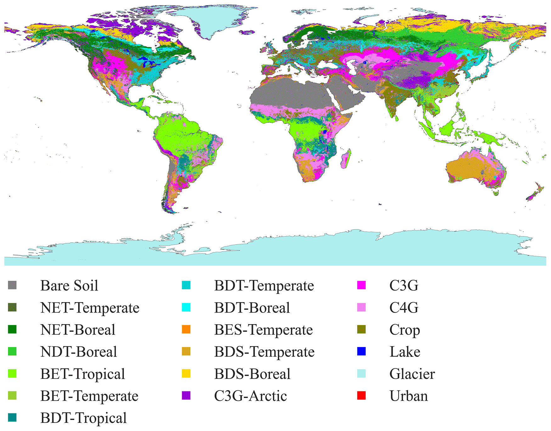
Figure 2Global LULC distribution in the year 2010. PFT abbreviations include the following: bare soil (Bare Soil); needleleaf evergreen trees in temperate (NET-Temperate) and boreal (NET-Boreal) regions; needleleaf deciduous trees in boreal regions (NDT-Boreal); broadleaf evergreen trees in tropical (BET-Tropical) and temperate (BET-Temperate) regions; broadleaf deciduous trees in tropical (BDT-Tropical), temperate (BDT-Temperate), and boreal (BDT-Boreal) regions; broadleaf evergreen shrubs in temperate regions (BES-Temperate); deciduous shrubs in temperate (BDS-Temperate) and boreal (BDS-Boreal) regions; C₃ grass in arctic (C3G-Arctic) and general (C3G) varieties; C₄ grass (C4G); crops (Crop); lake (Lake); glacier (Glacier); and urban (Urban).

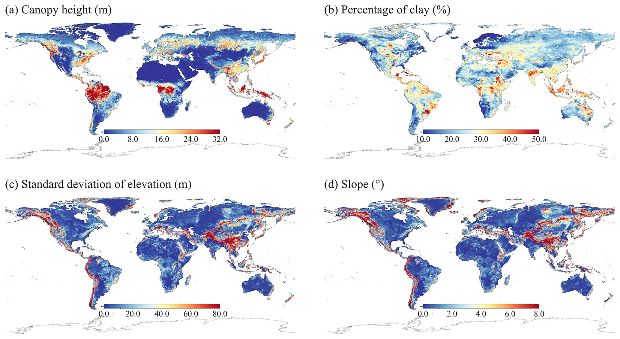
Figure 3Demonstration of global 1 km datasets (a) canopy top height, (b) percent clay, (c) standard deviation of elevation, and (d) slope.

4.2 Comparison between new and existing land surface parameters

The global distributions of different PFTs show varying degrees of difference when comparing the new parameters with the K2012 and ELM2/CLM5 default parameters (Figs. 4 and S1–S16 in the Supplement). Predominant types such as bare soil, BET-Tropical tree, C₃ and C₄ grasses, and crop are found consistently across all datasets. Notable differences include less bare soil in the new parameters and K2012 compared to the ELM2/CLM5 default, especially in high-latitude North America, western USA, southern Africa, central Asia, and central Australia (Fig. S1). While the new NDT PFT shows larger coverage in Siberia than K2012 and ELM2/CLM5 (Fig. S4), the BET-Tropical PFT is more prevalent in the new parameters across Central and South America (Fig. S5). The BET-Temperate PFT has greater area coverage in southern China in the new parameters (Fig. S6). For BDT-Tropical, BDT-Temperate, and BDT-Boreal PFTs, both the new and ELM2/CLM5 default parameters surpass K2012 data in coverage (Figs. S7–S9). The coverage of the new BDS-Temperate PFT is smaller than K2012 but larger than the ELM2/CLM5 default (Fig. S11), and the new BDS-Boreal PFT is less extensive in the boreal Northern Hemisphere compared to both K2012 and the ELM2/CLM5 defaults (Fig. S12). The C₃-Arctic PFT shows larger areas in the new parameters, particularly in northern Canada, with the new C₄ grass PFT being similar to that of K2012 and larger than ELM2/CLM5 C₄ grass. The crop PFT is less extensive in the new parameters, particularly in southeastern China, Europe, South America, Africa, and Australia.

Figure 4The global average area fractions of PFTs for three land surface parameter datasets. PFT abbreviations used on the x axis are displayed in Fig. 2.

Download

The global distributions of non-vegetated land covers of lake, glacier, and urban areas vary among the datasets (Figs. S17–S19). The new dataset shows slightly less lake coverage than K2012, but both are smaller than the ELM2/CLM5 default, particularly in high-latitude North America (Fig. S17). Glacier coverage in the new parameter is around 0.7 % smaller than K2012, with noticeable differences in the Arctic North America, while the ELM2/CLM5 default shows more extensive glacier coverage in Antarctica (Fig. S18). Regarding urban areas, K2012 has the smallest urban coverage in the Northern Hemisphere compared to both the new dataset and the ELM2/CLM5 default (Fig. S19). Meanwhile, the ELM2/CLM5 default exhibits more expansive urban areas in India and China than the new dataset and K2012.

The global annual mean LAI exhibits similar spatial patterns among the new parameter, K2012, and ELM2/CLM5 (Fig. 5). The overall global mean LAI for the new parameter (1.28 m² m⁻²) is slightly higher than that of K2012 (1.14 m² m⁻²) and the ELM2/CLM5 default data (1.24 m² m⁻²). In terms of spatial pattern, the new LAI, relative to K2012 (Fig. S20a), shows lower values in the NET-Boreal PFT over the Northern Hemisphere but higher values in the BET-Tropical PFT over the tropics. Similarly, compared with the ELM2/CLM5 default LAI (Fig. S20b), the new LAI also presents smaller values in both the NET-Boreal and NDT PFTs over the Northern Hemisphere but larger values in the BET-Tropical PFT regions.

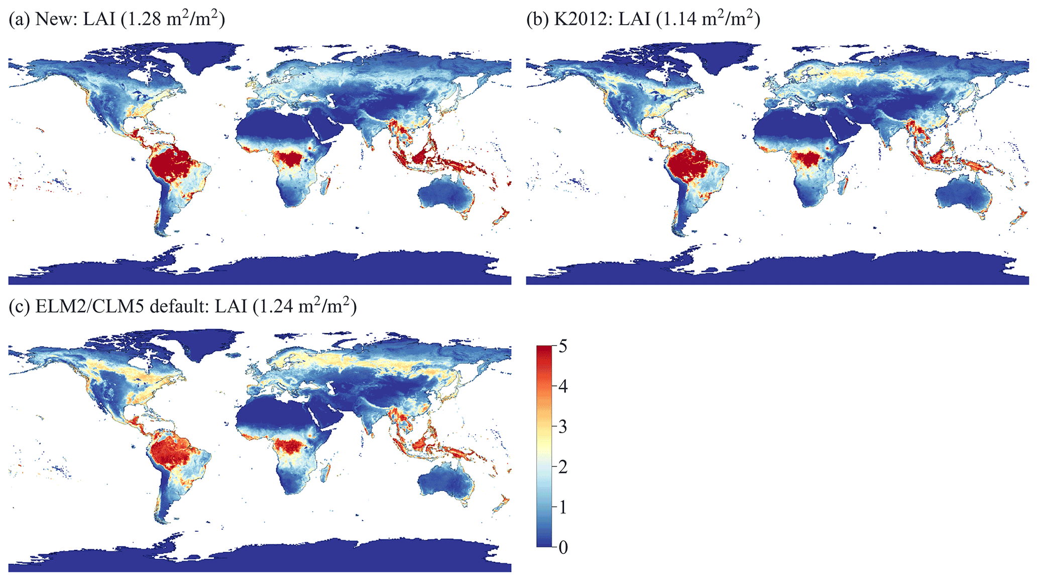
Figure 5Comparison of global annual mean LAI for (a) new, (b) K2012, and (c) ELM2/CLM5 default parameters. The global average is indicated in the panel title.

Soil parameters exhibit significant differences between the new and ELM2/CLM5 default datasets (Figs. 6a–c, S21, and S22). The global mean absolute differences between the new and ELM2/CLM5 default for percent sand, percent clay, and organic matter are 14.1 %, 8.1 %, and 30.5 kg m⁻³, respectively. Generally, the new soil parameters are spatially distributed more smoothly than those from ELM2/CLM5 with more patchy patterns (Fig. 6a vs. Fig. 6b). Specifically, the new percent sand is higher in regions like Europe, Siberia, southern Africa, and southern Australia but lower in areas such as the lower Mississippi River basin, northern Africa, and central and southeastern Asia (Fig. 6c). The new percent clay shows larger values in the western USA, northern Africa, central Asia, and Australia but smaller values in Alaska and eastern Europe (Fig. S21). For organic matter, the new parameter indicates smaller values in the Northern Hemisphere but larger values in other global regions compared to the ELM2/CLM5 default (Fig. S22).

Figure 6Comparisons of percent sand and slope. (a) New and (b) ELM2/CLM5 default percent sand, along with (c) their difference (new – ELM2/CLM5 default) for percent sand; (d) new, (e) ELM2/CLM5 default, and (f) their difference for slope. The global average is shown in the panel titles, with the global average of the absolute difference provided for (c) and (f).

Topography-related parameters exhibit broadly similar spatial patterns but with notable differences between the new and the ELM2/CLM5 default parameters, as seen in Figs. 6d–f and S23. The new slope parameter generally shows a larger slope relative to the ELM2/CLM5 default, particularly in mountainous regions (Fig. 6f). This could be attributed to the new 1 km slope being calculated from a finer 90 m resolution elevation. Differences in elevation between the new and ELM2/CLM5 parameters are more pronounced in areas such as various mountainous regions, Greenland, the Amazon Basin, the Tibetan Plateau, and Australia (Fig. S23).

4.3 Demonstration 1 km simulation over CONUS

ELM simulations at a 1 km resolution display significant spatial heterogeneity over CONUS (Fig. 7). The values of SM, LH, ELR, and ASR across CONUS follow approximately normal distributions, with averages of 0.3 m³ m⁻³, 39.0, 371.7, and 156.7 W m⁻², respectively (as shown in the histogram plots in Fig. 7). SM shows drier conditions over the west and southwest and wetter conditions over the US Midwest, Corn Belt, Mississippi River basin, and US Northeast (Fig. 7a). LH shows high values over the central and southeast and lower values over the west and southwest (Fig. 7b). The ELR generally shows higher values over regions with high surface temperature in the south (Fig. 7c). The ASR shows higher values over the southwestern regions determined by incoming solar radiation and albedo (Fig. 7d). Despite the high-resolution heterogeneity shown at 1 km resolution, we can still see the spatial patterns distinguished at coarse resolution, i.e., 0.5°×0.5°. These coarser footprints are from the GSWP3 atmospheric forcing with 0.5° resolution. As concluded by Li et al. (2022), atmospheric forcing is one primary heterogeneity source for land surface modeling. Therefore, k-scale atmospheric forcing needs to be developed to further advance k-scale offline land surface modeling.

Figure 7The annual mean of 1 km simulations of (a) SM, (b) LH, (c) ELR, and (d) ASR over CONUS. The 0.5°×0.5° boxes marked as L1, L2, L3, and L4 in (a) and (b) are selected to demonstrate the spatial scaling analysis. The inserted histogram plot illustrates the distribution of ELM2 simulations.

4.4 Demonstration of spatial scaling across scales

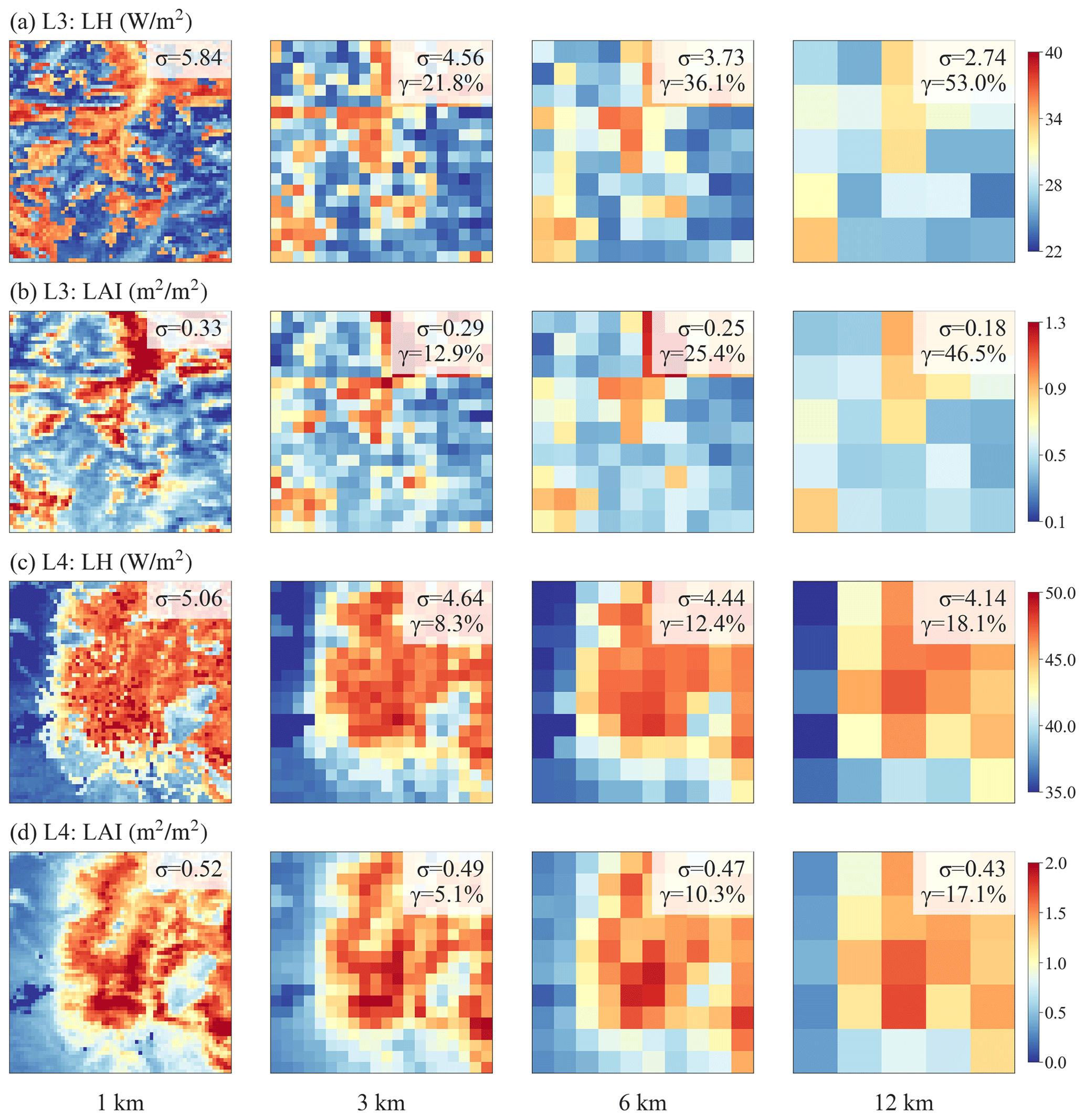
We next demonstrate the relationships between spatial variabilities and spatial scales for SM and LH. Four locations (in Fig. 8a and b) are specifically chosen to showcase varying levels of spatial information loss: L1 and L3 demonstrate a relatively large loss for SM and LH, respectively, while L2 and L4 represent a relatively small loss for SM and LH, respectively.

At location L1 (Fig. 8a), when the 1 km simulation is upscaled to coarser resolutions (i.e., larger spatial scale ratios), the spatial variability of SM decreases, resulting in a negative slope of β. As shown in Fig. 9a, compared to the original 1 km resolution, the information loss γ reaches up to 54.9 % at the 12 km spatial scale. The spatial pattern of SM is consistent with the spatial pattern of percent clay (Fig. 9a vs. Fig. 9b and Fig. 9c vs. Fig. 9d), indicating that soil texture contributes significantly to the spatial variability of SM. However, SM has a more negative β than the percent clay ($\mathit{\beta }=-\mathrm{0.28}$ vs. −0.19 at L1, as shown in Fig. 8a), suggesting that SM variability is amplified likely by other processes that are also influenced by soil texture. In contrast to location L1, location L2 exhibits less negative β values for both SM and percent clay, suggesting that their spatial variabilities exhibit less scale dependence (Figs. 8a and 9c, d). Both SM and percent clay at location L2 approximately maintain their spatial patterns of high values in the west and low values in the east across spatial scales (Fig. 9c and d).

Figure 8The scaling of spatial variabilities for (a) SM and percent clay and (b) LH and LAI. Both the x axis and y axis are in logarithmic scale. The slope of the linear regression line, β, quantifies the strength of the negative relationship between spatial scale and spatial variability. A more negative β value indicates a higher spatial-scale dependency and increased information loss at coarser spatial scales. Four 0.5°×0.5° boxes (displayed in Fig. 7), namely, L1 to L4, are chosen to contrast larger and smaller negative β values for SM and percent clay (L1 and L2) and for LH and LAI (L3 and L4).

Download

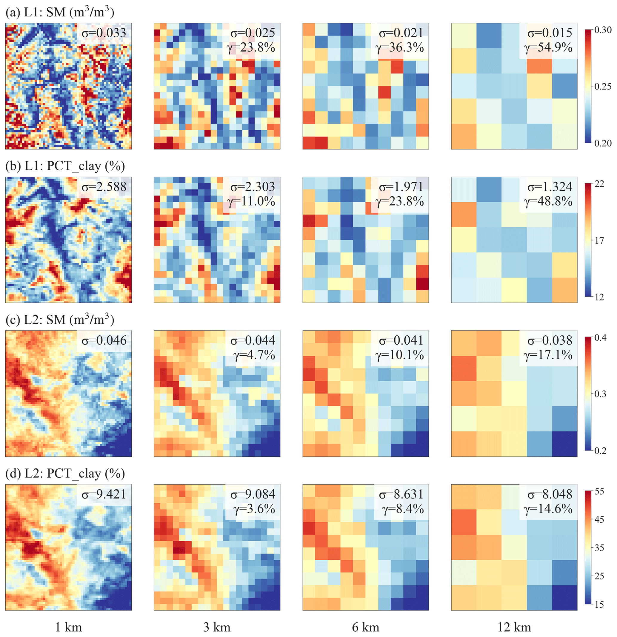
Figure 9Comparison of SM and percent clay across spatial scales at locations L1 and L2 highlighted in Fig. 7. Each panel displays the spatial patterns of SM or percent clay within a 0.5°×0.5° box, with the σ and γ presented in the legend.

Download

For LH, there is a more negative β value at location L3 than at location L4 ($\mathit{\beta }=-\mathrm{0.27}$ at L3 vs. −0.08 at L4, as shown in Fig. 8b), which indicates a larger decrease of spatial variability across spatial scales and lower variability persistence at location L3 than location L4 (Fig. 10). The spatial pattern of LH is consistent with the spatial pattern of LAI (Fig. 10a vs. Fig. 10b and Fig. 10c vs. Fig. 10d) at different spatial scales, suggesting that vegetation plays a significant role in the spatial variability of LH. Similar to comparison between SM and soil texture, LH has a more negative β than LAI (Fig. 8b).

Figure 10Similar to Fig. 9, but for LH and LAI at locations L3 and L4.

Download

4.5 The spatial variability of water and energy simulations and their drivers

We quantified the spatial variability simulated at 1 km resolution using σ within each 0.5°×0.5° box across CONUS. Four ML models were built to explore the spatial relationships between σ and its potential drivers, including σ of the land surface parameters and the temperature and precipitation averaged over the grid box. Overall, the ML models performed well in predicting the σ of the simulated variables, with small root mean square error (RMSE) and large R² (see Fig. S24). SM shows larger spatial variability in the US Southern Coastal Plain, lower Mississippi River, US Northeast, US Southeast, and regions around the Great Lakes (Fig. 11a), which is roughly consistent with the spatial heterogeneity of the high-resolution SM simulation in Vergopolan et al. (2022). Based on the SHAP method, the spatial variability of SM across CONUS is driven by various factors, mainly including the spatial variabilities of percent sand and percent clay, mean precipitation, the σ and μ of soil organic matter, the σ of canopy height, and mean temperature (Fig. 11b). Mean precipitation and temperature reflect climate conditions (Fig. S26), which are related to the water supply and water demand of soil water content. The spatial heterogeneity of soil properties, such as texture and organic matter content, affects soil hydraulic properties and generate more spatially variable soil water content. Vegetation characteristics, such as canopy height and LAI, could influence SM spatial variability through their effect on roughness length and rooting depth.

Figure 11The spatial variability over each 0.5°×0.5° grid cell (a, c, e, g) and the top eight most important drivers (b, d, f, h) of the spatial variability for SM, LH, ELR, and ASR. The inserted histogram plot illustrates the probability distribution of the spatial variability across CONUS. The relative importance of each variable in determining the spatial variability is calculated as the ratio of the mean |SHAP value| of the variable to the sum of the mean |SHAP value| of all variables. Therefore, the sum of the relative importance of all variables is 100 %.

The spatial variability of LH is large in the southeastern, central, and western mountainous regions of the USA (Fig. 11c). Vegetation properties and climate conditions mainly drive the variability of LH (Fig. 11d). The μ and σ of LAI can affect transpiration and soil evaporation, while canopy height can influence surface roughness length and, in turn, evapotranspiration. Mean precipitation and temperature reflect the overall climate conditions related to the water and energy available for latent heat.

ELR and ASR exhibit large spatial variability mainly over the western USA, with ASR additionally showing significant spatial variability across northern USA (Fig. 11e and g). This variability is primarily driven by climate conditions such as mean precipitation and temperature, topographic features such as standard deviation of elevation and slope, and vegetation properties including LAI and canopy height (Fig. 11f and h). These factors are related to the radiation input and surface properties, such as albedo and roughness length, which impact the energy cycles and availability of ELR and ASR.

4.6 The information loss of water and energy simulations and their drivers

We also evaluated the information loss in simulations when upscaling from 1 to 12 km resolution and analyzed the drivers of their spatial patterns over CONUS. Four ML models were built to explore the relationships between the γ of the simulations and its drivers, including the γ of the land surface parameters and the mean temperature and precipitation averaged over the 0.5°×0.5° box. These ML models performed well in predicting the simulations' γ, with small RMSE and large R² (Fig. S25).

Significant information loss ranging from 31 % to 54 % with maximum values exceeding 90 % is observed for SM, LH, ELR, and ASR simulations (Fig. 12). Their spatial patterns and drivers show distinct variations; γ_SM is primarily driven by the information loss of percent clay and sand, mean soil organic matter, and mean temperature, which affects the soil hydraulic properties and soil water balance (Fig. 12a and b). γ_LH displays high values in the eastern USA and low values in the western USA (Fig. 12c). It is primarily contributed by the information loss of vegetation properties such as LAI and canopy height, as well as mean LAI, which influences the partitioning of LH and sensible heat, and the partitioning of transpiration and evaporation (Fig. 12d). γ_ELR exhibits high values in the central and eastern USA, particularly in the northeastern USA, while γ_ASR has high values almost all over the USA, especially in the eastern regions (Fig. 12e and g). γ_ELR and γ_ASR are largely driven by vegetation properties such as LAI and canopy height, which are associated with energy processes such as albedo (Fig. 12f and h). Additionally, topography factors of standard deviation of elevation and slope also slightly contribute to γ_ASR.

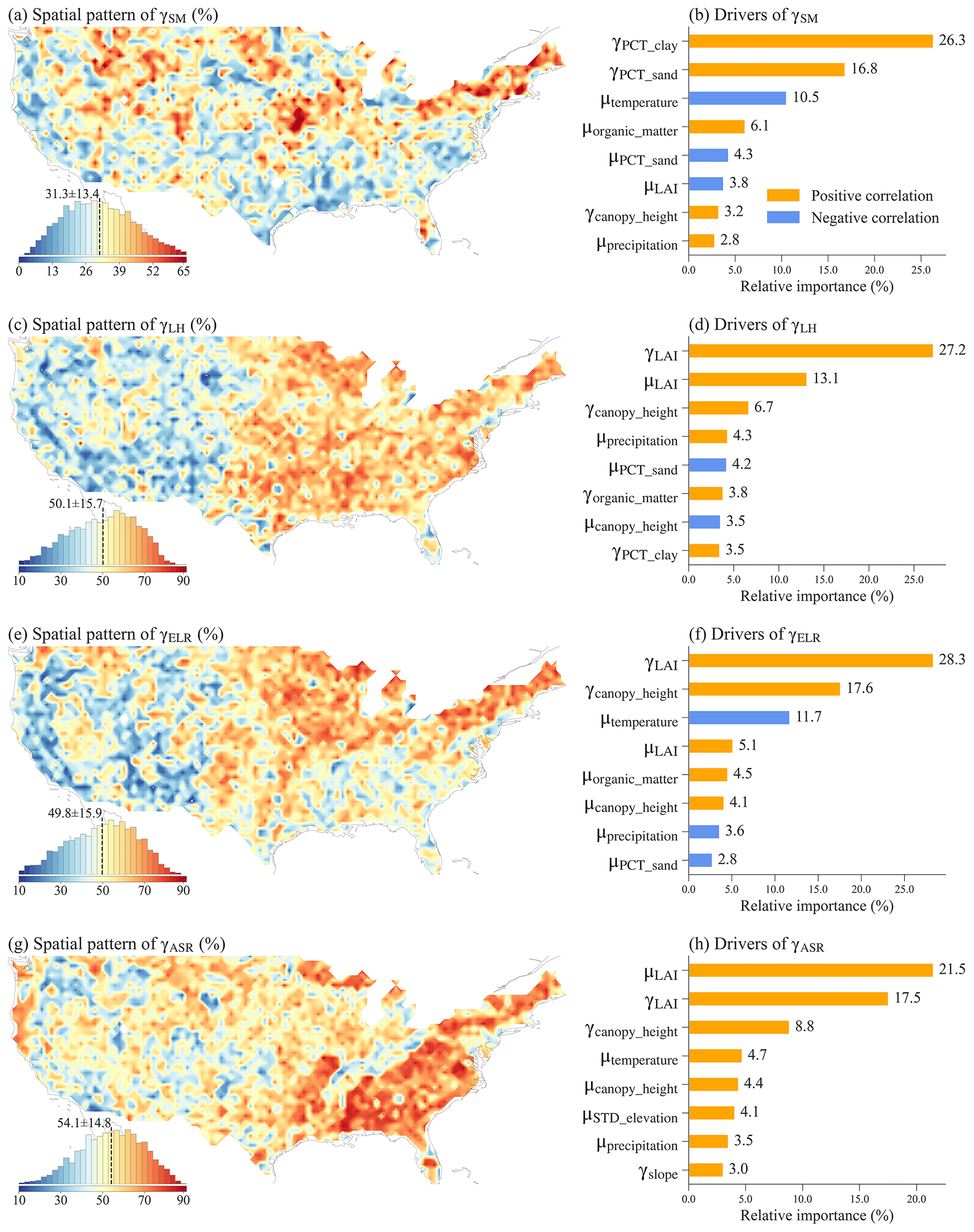
Figure 12Same to Fig. 11 but for information loss.

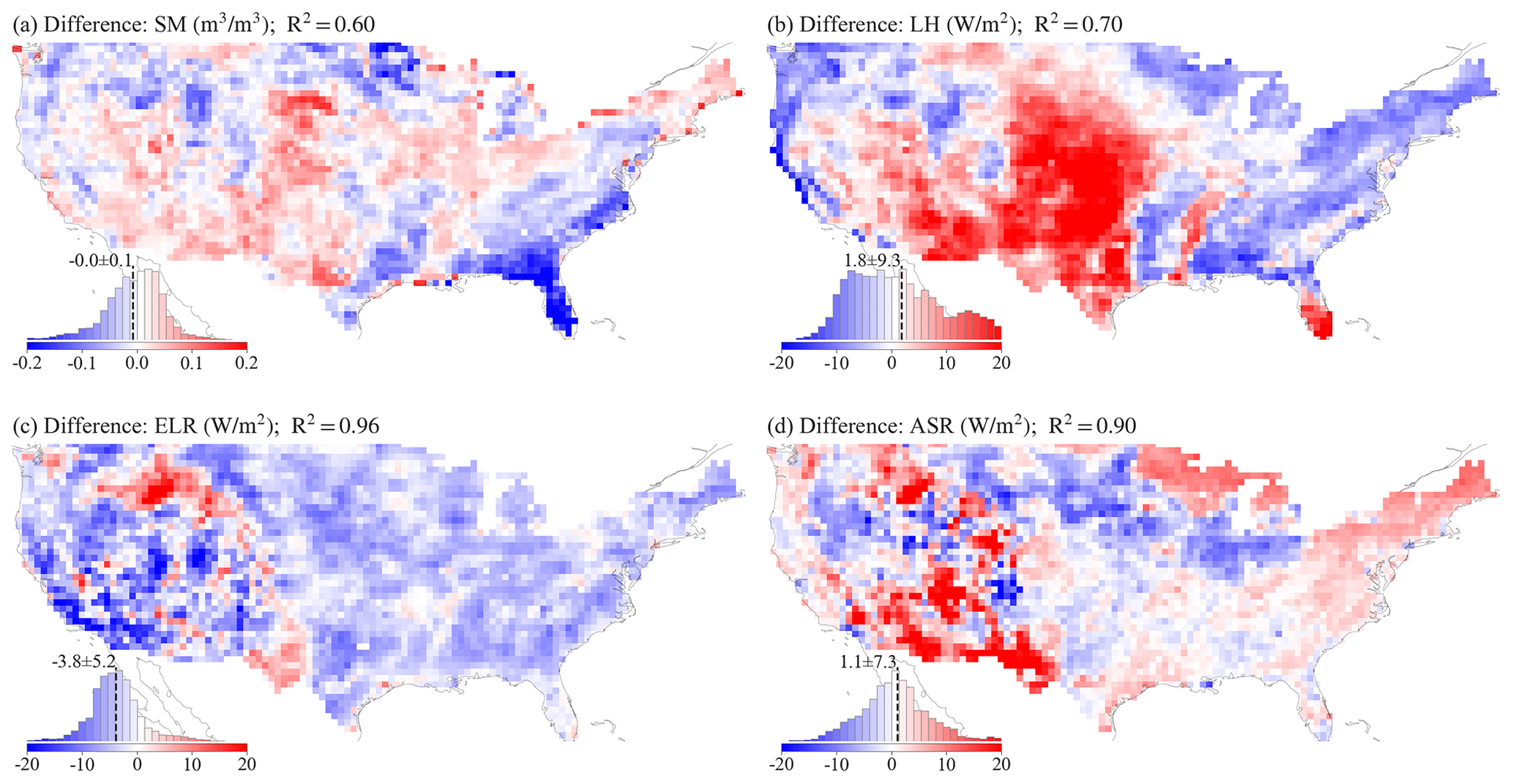
Figure 13Annual mean bias between ELM-simulated variables and reference datasets over CONUS: (a) SM, (b) LH, (c) ELR, and (d) ASR. The negative values indicate lower ELM values compared to the reference data. The inserted histogram plot illustrates the distribution of grid values. For spatial patterns of the reference datasets, refer to Fig. S27. The correlation coefficient (R²) between the ELM simulation and the reference dataset is calculated and displayed in the title of each panel.

4.7 Comparison of ELM simulation against reference data

The average spatial biases between ELM and reference datasets across CONUS are relatively small, with SM bias at −0.01 m³ m⁻³, LH bias at 1.8 W m⁻², ELR bias at −3.8 W m⁻², and ASR bias at 1.1 W m⁻² (Figs. 13 and S27). The correlation coefficient (R²) between ELM and reference datasets was relatively high at 0.60 (for SM), 0.70 (for LH), 0.96 (for ELR), and 0.90 (for ASR). However, the spatial distribution of these biases exhibits variability, with some areas showing more pronounced biases than others. Specifically, in comparison with GLEAM SM, ELM tends to underestimate SM in the southeastern Texas and across the eastern and southeastern CONUS, while it overestimates SM in the western, central, and southwestern CONUS, including the central-eastern USA, which are primarily agricultural areas. For LH, ELM simulates higher values than the MODIS LH dataset in the western and central USA and Florida but lower values in regions such as the eastern and northeastern CONUS, the western US coastal areas, and the US Pacific Northwest. Regarding radiation variables, ELM generally underestimates ELR across nearly all of CONUS and tends to overestimate ASR, particularly in the southwestern, southern, eastern, northeastern, and northern regions of CONUS.