


Abstract
Using a set of general-relativistic magnetohydrodynamics simulations that include proper neutrino transfer, we assess for the first time the role played by the fallback accretion onto the remnant from a binary neutron star merger over a timescale of hundreds of seconds. In particular, we find that, independently of the equation of state, the properties of the binary, and the fate of the remnant, the fallback material reaches a total mass of ≳10−3M⊙, i.e., about 50% of the unbound matter, and that the fallback accretion rate follows a power law in time with slope ∼t−5/3. Interestingly, the timescale of the fallback and the corresponding accretion luminosity are in good agreement with the so-called "extended emission" observed in short gamma-ray bursts (GRBs). Using a simple electromagnetic emission model based on the self-consistent thermodynamical state of the fallback material heated by r-process nucleosynthesis, we show that this fallback material can shine in gamma and X-rays with luminosities ≳1048 erg s−1 for hundreds of seconds, thus making it a good and natural candidate to explain the extended emission in short GRBs. Additionally, our model for fallback emission reproduces well and rather naturally some of the phenomenological traits of extended emission, such as its softer spectra with respect to the prompt emission and the presence of exponential cutoffs in time. Our results clearly highlight that fallback flows onto merger remnants cannot be neglected, and the corresponding emission represents a very promising and largely unexplored avenue to explain the complex phenomenology of GRBs.
Export citation and abstract BibTeX RIS

Original content from this work may be used under the terms of the Creative Commons Attribution 4.0 licence. Any further distribution of this work must maintain attribution to the author(s) and the title of the work, journal citation and DOI.
1. Introduction
The merger of binary compact objects is a complex phenomenon involving many different physical processes, making them a great laboratory for many branches of physics and astrophysics (Baiotti & Rezzolla 2017; Paschalidis 2017). Nonetheless, because the inspiral and merger processes are deterministic, any observable produced by this process has the potential of revealing the properties of the progenitor binary and, hence, of matter and gravity under extreme conditions. In particular, while the characteristics of the different outflows launched in the merger and their electromagnetic (EM) signals are fully determined by the properties of the binary, the self-consistent and long-term modeling of these events and their observational counterparts is extremely complex and currently cannot be performed without a number of approximations. The first binary neutron star (BNS) multimessenger merger event, GW170817, presented, in addition to gravitational waves, a rich set of EM counterparts: a weak short gamma-ray burst (GRB), a thermal kilonova transient, and a long-lasting afterglow associated with the relativistic jet launched by the remnant (Abbott et al. 2017a, 2017b; The LIGO Scientific Collaboration et al. 2017; D'Avanzo et al. 2018; Margutti et al. 2018; Mooley et al. 2018; Troja et al. 2018; Ghirlanda et al. 2019; Lamb et al. 2019; Makhathini et al. 2020) . This afterglow could be currently rebrightening in the X-rays and changing spectral index, possibly revealing another emission component (Balasubramanian et al. 2021; Hajela et al. 2022). Other EM counterparts are predicted from BNS mergers, such as an early X-ray flash (Fernández & Metzger 2016), but have not yet been observed. These EM signals from BNS mergers are part of the rich phenomenology of short GRBs that had been explored well before GW170817 (see, e.g., Berger 2014; D'Avanzo 2015). In this phenomenology, the so-called "extended-emission" episodes (Norris & Bonnell 2006)—that is, stretches of soft gamma-ray to hard X-ray emission that can last for hundreds of seconds after the prompt emission of short GRBs—are a particularly puzzling aspect and the main focus of this paper. It is important to note that the extended-emission component is clearly distinct from the prompt emission because of its softer spectrum, as well as from the afterglow. In their ensemble, all of these counterparts likely arise from distinct outflows from the merger, either at ultrarelativistic or at more moderate speeds—and the relative importance of these outflows is therefore determined by the properties of the progenitor binary.
In this rich but complex picture, the ideal tool to study the full sequence from merger to EM signals is first-principles general-relativistic magnetohydrodynamical (GRMHD) simulations of the merger followed by adequate postprocessing to implement the emission models of the EM counterparts. Studying the full picture from the binary properties to the EM signals has many advantages. First, using constraints on the binary system provided by low-latency analysis of the gravitational-wave data (such as the chirp mass) can guide follow-up searches of EM counterparts by partially predicting the expected signals. This has already been done for the kilonova signal (Barbieri et al. 2021; Nicholl et al. 2021) and should be extended to other counterparts, most notably, those detected in faraway or on-axis events expected for the future, such as the afterglow (see, e.g., Gill & Granot 2018; Lazzati et al. 2018; Duque et al. 2019; Gill et al. 2019; Hotokezaka et al. 2019; Troja et al. 2019; Wu & MacFadyen 2019; Beniamini et al. 2020, 2022; Nakar & Piran 2020; Ryan et al. 2020). An early prediction of EM counterparts would obviously be useful to optimize the follow-up searches and, in the third-generation detector era (Punturo et al. 2010), in which many BNSs will be detected per day (see, e.g., Ronchini et al. 2022), to choose the most promising systems EM-wise to focus the follow-up efforts on those. Second, studying existing catalogs of EM signals from BNS mergers, such as short GRBs and their afterglows, can help to constrain the progenitors of short GRBs and their formation channels. This approach, together with population studies, can constrain, for instance, the GRB-luminosity function (Ghirlanda et al. 2016) by linking it to the progenitor system parameters. Finally, ab initio calculations represent possibly the only way in which it may be possible to find conclusive answers to some of the most puzzling aspects of the EM phenomenology of short GRBs, such as the extended emission. Moreover, gravitational-wave-triggered events may enable us to probe the off-axis properties of the extended emission, which are mostly inaccessible through short GRB catalogs, but might be very useful in constraining the emission associated with these events.
We recall that the extended emission in the gamma-ray and X-ray bands covers two recurring features in the short GRBs observed. As already mentioned, the gamma-ray extended emission is characterized by an episode of gamma-ray emission that can last for hundreds of seconds after the prompt emission of short GRBs and that is of a lower luminosity and softer spectrum than the parent prompt (this is also referred to as the "spike"). Gamma-ray extended emission was first discovered in the prototypical GRBs 050724 and 060614 (Barthelmy et al. 2005a; Gehrels et al. 2006), which were initially classified as long GRBs because of their extended emission. Gamma-ray extended emission is present in 2%–25% of short GRBs, depending on the instrument and search method, and bursts with extended emission are characterized by very low spectral lags in the parent spike (Norris & Bonnell 2006; Kaneko et al. 2015), consistent with those of short GRBs. Short GRBs with and without detectable extended emission are indistinguishable in terms of galactic offset and host galaxy properties (Fong et al. 2022; Nugent et al. 2022), consistent with them arising from the same progenitor systems, perhaps with particular characteristics.
On the other hand, the extended emission in the X-ray band was discovered in a sample of Swift short GRBs with early X-ray observations and extended gamma-ray observations (Kagawa et al. 2015). These authors concluded from a restricted sample that the extended near-flat X-ray emission was the X-ray counterpart of the extended emission in the gamma rays. The X-ray extended emission has a similar duration (up to hundreds of seconds) and, within the sample studied, featured an exponential cutoff. As a possible and simple mirror of the extended emission in gamma rays, X-ray extended emission was studied per se and found in approximately 20%–50% of short GRBs detected by Swift (Kisaka et al. 2017; Kagawa et al. 2019). In short GRBs with measured redshift, the luminosities of extended-emission episodes in X-rays span from 1046 to 1049 erg s−1 in the Swift X-Ray Telescope (XRT) band (Kisaka et al. 2017). It should be remarked that the fraction of the total energy lost in a short GRB with extended emission that is output in the extended-emission episode varies widely (Perley et al. 2009; Bostancı et al. 2013; Kagawa et al. 2019), and the extended-emission episode itself can largely exceed the fluence of the prompt emission, suggesting a large reservoir of energy active on long timescales.
Extended emission in short GRBs has been interpreted through various pictures. The list of proposed models today includes dissipation in a second jet launched by the black hole central engine through disk accretion (Barkov & Pozanenko 2011; Gottlieb et al. 2023), through material falling back after the burst (Kisaka & Ioka 2015) (with r-process heating in the fallback material being sometimes taken into account; Metzger et al. 2010; Desai et al. 2019), or from a magnetar central engine (Bucciantini et al. 2012). Magnetar models also consider the relativistic wind as a potential source (Metzger et al. 2008; Murase et al. 2018), acceleration of a fallback accretion disk through magnetic propelling (Gompertz et al. 2013, 2014, 2023), or the interaction of the slow and fast winds launched respectively before and after the dissipation of the differential rotation of the merger remnant (Ciolfi & Siegel 2015; Rezzolla & Kumar 2015). Scenarios invoked for longer-duration soft episodes of long GRBs or of flares in GRB afterglows can likely be adapted to extended emission in short GRBs (see, e.g., Lee et al. 2009; Gao et al. 2022).
The ejection of material that remains gravitationally bound to the central object and falls back on long timescales seems to be ubiquitous in explosive events. Such material is invoked in various contexts, from tidal disruption events (TDEs) with a mostly tidal component (Krolik & Piran 2012) to BNS mergers considering secular ejecta (Ishizaki et al. 2021a). The dynamics of such material has attracted much attention, starting from the early analytical studies prescribing the distribution of energy in the debris (Rees 1988), notoriously leading to a simple mass accretion rate scaling as ∼t−5/3 with time, to numerical relativity simulations that have refined this picture under more realistic conditions (see, e.g., Rosswog 2007). TDEs, in particular, have a rich observational history, with X-ray signatures following the ∼t−5/3 accretion rate to more complex phenomenology hinting at the launching of jets (see, e.g., Komossa 2015).
For BNS mergers, the picture for fallback material is somewhat complicated by the presence of various ejecta (that are either dynamical or secular; Gill et al. 2019), the nature of the remnant compact object (which can be either a massive neutron star or a black hole; Nathanail et al. 2021b), and the interaction of the jet with the ejected material (Murguia-Berthier et al. 2016; Hamidani et al. 2020; Urrutia et al. 2021; Nathanail et al. 2021a; Gottlieb et al. 2022; Kiuchi et al. 2023; Mpisketzis et al. 2024). Recently, Metzger & Fernández (2021) and Ishizaki et al. (2021a) have sought to explain the putative excess in the afterglow of GW170817 with the emission of fallback material from the secular ejecta. Furthermore, Ishizaki et al. (2021b) have studied the impact of nuclear reaction reigniting in the fallback accretion, showing a halt in the accretion flow due to the internal heating. However, while interesting, these studies lack a first-principles insight into the amount of bound ejecta and on the fallback dynamics starting from the merger phase, as well as a study of the emission from this material in the shorter timescales relevant for extended emission.
One of the main scopes of this paper is to improve on these studies by using state-of-the-art GRMHD simulations with proper neutrino transport followed by a semianalytical treatment of the fallback dynamics to study in detail the fallback accretion and the radiation arising from this inflow. This allows us to explore the possibility that extended emission can be attributed to this fallback material. We contrast the properties of this emission component according to the mass ratio and equation of state (EOS) of the material assumed in the neutron stars in a first search for phenomenological trends with binary characteristics. In this way, we find that the amount of bound matter is substantial, being almost 50% of the dynamically unbound matter and reaching a total of ≳10−3 M⊙. Furthermore, the accretion rate follows a universal power law in time with slope ≃t−5/3, which is independent of the EOS, the properties of the binary, and the fate of the remnant. Importantly, the timescale of the fallback and the corresponding accretion luminosity all are in good agreement with the long-term emission observed in short GRBs. Using a simple EM emission model based on the thermodynamical state of the fallback material heated by r-process nucleosynthesis, we show that this fallback material can shine in the gamma and X-rays with luminosities ≳1048 erg s−1 for hundreds of seconds, thus making it a good candidate to explain the extended emission and reproducing rather naturally some of the phenomenological traits of extended emission, such as its softer spectra with respect to the prompt emission and the presence of exponential cutoffs in time.
The plan of the paper is as follows. Section 2 presents the framework of our numerical simulations, including the choice of the binary systems we simulate, as well as a description of the material ejected from the mergers we simulate. Section 3 presents our semianalytical model to predict the dynamics of the fallback of the bound material ejected and the radiation emitted by this fallback flow. In Section 4, we present our finding of this fallback radiation as a new high-energy emission component of BNS mergers, and we discuss this component in relation to the observations of extended-emission episodes of short GRBs. In Section 5, we conclude with an outlook of the role of this fallback radiation in other long-lasting high-energy signals such as X-ray plateaus.
2. Binary Mergers and Fallback Material
2.1. Numerical Setup
As mentioned in the Introduction, what distinguishes our work from similar studies in the literature is the realistic modeling of BNS mergers so as to have not only an accurate description of the matter ejection on the nonlinear physics involved in the merger but also an accurate dependence of the fallback dynamics on the properties of the binaries. To this scope, we have considered four representative binaries described by two different and temperature-dependent EOSs. The first one is the SFHO EOS (Hempel & Schaffner-Bielich 2010), which is based on relativistic mean field calculations and predicts a maximum nonrotating Tolman–Oppenheimer–Volkoff (TOV) mass of MTOV ≃ 2.06 M⊙; the second EOS is the TNTYST (Togashi et al. 2017), which is based on the variational many-body theory and instead allows for higher masses, with MTOV ≃ 2.23 M⊙. For all four binaries, the total gravitational mass at infinite separation exceeds the expected maximum mass for a uniformly rotating remnant with their respective EOSs assuming a ratio  (Breu & Rezzolla 2016; Musolino et al. 2024). On the other hand, all the binaries have the same chirp mass corresponding to the estimated value for the GW170917 event (Abbott et al. 2017b), and considering M2 (M1) to be the gravitational mass of the secondary (primary) star in the binary, we consider two different mass ratios q:=M2/M1 ≤ 1, namely, q = 1.00 and q = 0.75, to model either an equal or an unequal-mass merger. Overall, this choice of EOS and mass ratio allows us to explore and contrast the scenarios modeled by the simulation in which the merger remnant remains a hypermassive neutron star (HMNS) from the one in which it collapses to a black hole a few millisecond after the merger. Details on the properties of the four binaries considered and of their outcome can be found in Table 1.
Table 1. The Four BNS Systems Considered in This Study, with Binary Parameters and General Characteristics of the Fallback Episodes
| M1 | M2 | q | EOS | tcoll | Remnant | Mrem | mtot | mFB | mKN | mFB/mKN | |
|---|---|---|---|---|---|---|---|---|---|---|---|
| (M⊙) | (M⊙) | (ms) | (M⊙) | (M⊙) | (M⊙) | (M⊙) | (%) | ||||
| SFHO-q1.0 | 1.36 | 1.36 | 1.00 | SFHO | 3.7 | Black hole | 2.63 | 8.62 × 10⁻³ | 1.60 × 10⁻³ | 7.02 × 10⁻³ | 23 |
| SFHO-q.75 | 1.18 | 1.57 | 0.75 | SFHO | 4.0 | Black hole | 2.64 | 1.04 × 10⁻² | 3.48 × 10⁻³ | 6.92 × 10⁻³ | 50 |
| TNTYST-q1.0 | 1.36 | 1.36 | 1.00 | TNTYST | ⋯ | HMNS | 2.68 | 9.97 × 10⁻³ | 3.76 × 10⁻³ | 6.21 × 10⁻³ | 60 |
| TNTYST-q.75 | 1.18 | 1.57 | 0.75 | TNTYST | ⋯ | HMNS | 2.78 | 1.33 × 10⁻² | 4.05 × 10⁻³ | 9.25 × 10⁻³ | 44 |
Note. M1, M2: masses of the component neutron stars in the binary. q = M1/M2 < 1: mass ratio of the binary. tcoll: in the case where a black hole forms in the simulation domain, time of formation after merger. Mrem: mass of the remnant compact object of the merger. mtot: total mass ejected from premerger to postmerger phases. mFB: mass of bound material ejected. mKN: mass of unbound material ejected, thus denoted for its role in the kilonova signal.
Download table as: ASCIITypeset image
As mentioned earlier, the evolution of the four binaries is carried out making use of the state-of-the-art numerical 3+1 code suite developed in Frankfurt, which consists of the FIL code for the higher-order finite-difference solution of the GRMHD equations using high-resolution shock-capturing methods (Toro 1999; Rezzolla & Zanotti 2013) and a fourth-order accurate conservative finite-difference scheme (Del Zanna et al. 2007). The evolution of the spacetime is instead carried out with the Antelope spacetime solver (Most et al. 2019), which solves the constraint damping formulation of the Z4 formulation of the Einstein equations (Bernuzzi & Hilditch 2010; Alic et al. 2012). The code suite evolves the full set of equations in conjunction with the EinsteinToolkit (Loeffler et al. 2012; Zlochower et al. 2022), exploiting the Carpet box-in-box adaptive mesh refinement (AMR) driver in Cartesian coordinates (Schnetter et al. 2006),
In addition, to accurately capture the temperature and composition of the ejected and bound material, the effect of weak interactions needs to be properly included. We do so by employing the recently developed code FIL-M1 (Musolino & Rezzolla 2024), which employs a moment-based neutrino-transport scheme. More specifically, FIL-M1 evolves the first two moments of the energy-integrated Boltzmann equations for neutrinos using standard, second-order, finite-volume, high-resolution shock-capturing methods. Thanks to the moment-based radiation transport scheme, we are able to include all the leading-order weak reactions in our simulations, thereby accounting for neutrino heating and cooling and momentum transfer, as well as the composition changes resulting from weak interactions.
All our simulations are performed on a grid spanning Ω = [−1500, 1500]3 km with seven fixed levels of refinement and the grid spacing on the finest level being dx = 310 m. Moreover, we include the effect of magnetic fields in all our simulations, initializing it as a purely poloidal magnetic field confined inside the stars, with a maximum initial strength of ≃1016.5 G for the equal-mass systems SFHO-q1.0 and TNTYST-q1.0, ≃1016.7 G for SFHO-q.75, and ≃1015 G for TNTYST-q.75 (see Chabanov et al. 2023 for a recent discussion of why magnetic fields confined to the crust are not likely). This value, despite being much larger than what would be expected for old neutron stars at the end of their inspiral, has a corresponding magnetic energy that is much smaller than the binding energy of the system and hence does not significantly affect the dynamics of the system before merger (see, e.g., Giacomazzo et al. 2009). In addition, and as is customary in this type of simulation, starting with an unrealistically large magnetic field allows us to better capture realistic magnetic field values after the BNS merger despite our resolution being insufficient for correctly capturing the dynamical magnetic field amplification due to the Kelvin–Helmholtz instability.
2.2. Bound and Unbound Material
Clearly, a very important aspect of our research consists of properly distinguishing matter that is gravitationally bound from matter that is not and hence will not fall back onto the merger remnant. To this scope, and as is customary in these simulations, we construct a matter "detector" consisting of a spherical surface at a distance Rd = 300 M⊙ from the center of coordinates and record the properties of the matter flowing out of such a 2-sphere. In particular, we use the covariant time component of the material's four-velocity ut to determine the matter that is gravitationally bound (i.e., ut > −1) or unbound (i.e., ut < −1). We favor this criterion, which is also referred to as the "geodesic criterion," over the other common alternative represented by the so-called "Bernoulli criterion," hut > −1 (Rezzolla & Zanotti 2013), where h is the specific enthalpy, because the pure kinematic quantity ut relates directly to the subsequent dynamics of the bound material in the gravitational field of the remnant that we will use to determine the fallback time below. We note that, in principle, hydrodynamical processes can convert internal energy to kinetic energy, thus possibly unbinding material that was initially deemed bound through the ut criterion; similarly, matter that is considered unbound can undergo shock heating and become bound (see Bovard et al. 2017 for a discussion). However, as we will show in Section 2.3 by varying the position of the matter detector, the conversion of internal energy into kinetic energy does not occur in practice in our simulations, likely because of the small rest-mass density of the matter once it reaches the detector.
Because the dynamics of the bound matter outside of the detection sphere cannot be followed in detail (even if bound, the matter past the detector at Rd travels outward to distances that are orders of magnitude larger than Rd ), we model it in terms of geodesic motion in the gravitational field of the merger remnant. This is a reasonable assumption given that the rest-mass densities past the detector are comparatively very small (i.e., ρ ≲ 109 g cm−3), and hydrodynamical effects can be neglected. More importantly, and as we show in Section 2.4, the kinetic energy of the material detected decreases over the course of the postmerger evolution for all the systems studied. Thus, the material ejected at later times does not have the opportunity to collide with matter ejected earlier (potentially leading to shocks), so that we do not expect any interaction between the trajectories of the bound material.
A most important property of the bound matter is the time it will take to fall back onto the remnant. We could calculate this "fallback timescale" tFB in terms of the geodesic equations for the matter collected at the detector (and indeed we have done so), but a much simpler and computationally less expensive estimate can be obtained using simple and analytic Newtonian expressions. In particular, matter with four-velocity ut and specific angular momentum ℓ will have an orbit in the remnant's gravitational field with mass Mrem with specific energy

orbital eccentricity e

and orbit semimajor axis a

In general, in its motion from the detector surface away from the merger remnant and back, the ejected matter does not trace a full orbit, and the duration of its freefall orbit is given by

where the θ is the angle traced by the (planar) orbit and θs can be determined from a, e , and Rd (see, e.g., Rosswog 2007). This is the explicit solution to the Newtonian equation of motion in the gravity field of the central object.
However, we have the particular aim here of describing fallback flows on timescales of tens of seconds, much larger than the dynamical timescale around the central object. In this case, the duration of the fallback orbit is almost that of the full Newtonian orbit, whose period is

which is the well-known result of Newton's two-body problem.
Equations (4) and (5) ultimately represent an approximation of the actual fallback time that would be computed for the geodesic orbit of a massive test particle having the same energy and angular momentum moving in a Kerr spacetime with mass Mrem and dimensionless spin χrem. In Appendix A.2, we report a comparison between the fallback times computed with the two approaches. However, we can anticipate here that for long-period orbits, i.e., orbits with tFB ≳ 1 s, the differences between the Kerr geodetic estimate and the Newtonian estimate are always ≲0.2%, which is not surprising given that the orbits are mostly in a weak-field region where r/Mrem ≳ 200. Such an error is well below other uncertainties in our modeling, and given that Equation (4) comes with a considerable computational gain, it has been set as the method of choice in our analysis. Note that, by construction, we cannot monitor bound material with orbits that are totally contained within the detector 2-sphere. Stated differently, the fallback times we compute are necessarily larger than

which is much smaller than the typical timescales considered in our analysis but is useful to bear in mind when considering the discussion in Section 2.3.
What still needs to be determined is the mass Mrem of the remnant, which we obtain with two different methods providing comparable results. More specifically, in the case where a black hole forms within the simulation timescale, we determine the black hole mass using the quasi-local integral on the apparent horizon surface as determined by the vanishing of a null geodesic congruence expansion (Thornburg 1996; Dreyer et al. 2003). In the cases where the remnant is a metastable HMNS, we rely on the gravitational field measured at the detector surface. In particular, in a 3+1 decomposition of spacetime (see, e.g., Gourgoulhon 2007; Rezzolla & Zanotti 2013), the covariant tt metric component is given by

where α and βi are the lapse function and shift vector, respectively. On the other hand, in the weak-field approximation of general relativity, such a metric function at the detector surface 4 can be related to the Newtonian gravitational potential Φ as

so that

Equation (9) thus provides an independent measurement of the mass relevant for the fallback dynamics, including, in the case of black hole formation, the eventual accretion disk, though it is negligible in the cases studied here. The gravitational mass measured via Equation (9) in this method agrees almost exactly with the Arnowitt–Deser–Misner (ADM) mass in the simulation domain. By applying these two methods, we find their results to agree to within 2% for the two binaries where a black hole forms (see Table 1). For convenience, since it can be used equally well in the case of a black hole or HMNS, we will use the remnant mass computed via Equation (9) for all of the binary systems.
As a concluding remark, we note that to avoid oversampling the polar region of our spherical detectors while only having a few cells near the equator, as would be the case when using spherical coordinates to represent the discrete grid on the 2-sphere, we developed a code where the surface of the detector is discretized following the HEALpix scheme (Górski et al. 2005). 5 In this coordinate system, all the cells have the same surface area, and a lower overall resolution is sufficient to capture the relevant characteristics of the ejected matter as it crosses the detector.
2.3. Dynamics of the Bound Ejecta
In Figure 1, we present snapshots at representative times of the properties of the material crossing the detector sphere for the two SFHO binaries. For each column, the top hemispheres report the instantaneous rest-mass flux per unit solid angle  , while the bottom hemispheres show the values of ut
, with red (blue) shading marking matter that is gravitationally bound (unbound). The color bar for ut
was chosen to easily distinguish the bound material in red from the unbound material in blue. Above each panel, we report the times of the snapshots relative to the merger time, which, as is customary, is defined as the coordinate time at which the amplitude of the ℓ = m = 2 component of the gravitational-wave strain reaches its first maximum. In Figure 2, we present the same data for the two TNTYST binaries.
, while the bottom hemispheres show the values of ut
, with red (blue) shading marking matter that is gravitationally bound (unbound). The color bar for ut
was chosen to easily distinguish the bound material in red from the unbound material in blue. Above each panel, we report the times of the snapshots relative to the merger time, which, as is customary, is defined as the coordinate time at which the amplitude of the ℓ = m = 2 component of the gravitational-wave strain reaches its first maximum. In Figure 2, we present the same data for the two TNTYST binaries.

Figure 1. Snapshots of the material flowing through the detector surface at Rd = 300 M⊙ at various times of the simulation. Upper panels: SFHO-q1.0 system. Lower panels: SFHO-q.75 system. Upper hemispheres: mass flux per unit solid angle. Lower hemispheres: ut of the flowing material. The three columns correspond to different times during the evolution, as reported in Figure 3.
Download figure:
Standard image High-resolution image
Figure 2. Same as Figure 1 but for the two TNTYST binaries.
Download figure:
Standard image High-resolution imageWhile the properties of the ejected material in BNS mergers have been discussed in a number of papers (see, e.g., Sekiguchi et al. 2015; Bovard et al. 2017; Most et al. 2021; Camilletti et al. 2022; Papenfort et al. 2022), Figures 1 and 2 show rather clearly a feature that has not been remarked on sufficiently so far. More specifically, and irrespective of the mass ratio of the binary, the ejected material is initially mostly unbound (left column), and then the fraction of bound ejecta progressively increases (middle column) until a stage is reached where the ejecta is predominantly bound (right column). In addition, the geometrical distribution of the ejected matter is such that the front of the bound material progresses from the equatorial regions up to the polar directions, ending up by filling the whole sphere. Finally, while the early unbound ejecta is strongly anisotropic as a result of the tidal tails, the bound ejecta is quite isotropic. By comparing the upper and lower panels for each column, we find that the mass asymmetry in the binary increases the anisotropy in the polar direction of the early unbound ejecta (right column), as expected from its origin from the tidal tails, retaining such a property also at later times (right column). A more careful analysis of the polar distribution of the bound ejecta (not shown in Figures 1 and 2) reveals that the anisotropies are smaller than 15% for t − tmer ≳ 20 ms; i.e., for the bound matter, the mass flux differs by less than 15% across the radial directions at these times. Therefore, the bound ejecta can be considered as essentially isotropic at late times.
By contrasting Figures 1 and 2, we can appreciate the impact of the EOS and in particular the role played by the stiffness (the SFHO EOS is stiffer than the TNTYST). More specifically, when considering a softer EOS in Figure 2, we find that the transition from unbound to bound is still present, however to a lesser extent, where significant unbound flux is found even at later times in the high-latitude regions. Similarly, the distribution of bound material at intermediate and late times (middle and right columns) is less isotropic, with a clear presence of unbound material at very high latitudes as a result of a collimated outflow in the case of the TNTYST EOS. The origin of the slightly different behavior is to be found in the different nature of the remnant, which is a black hole in the case of the SFHO EOS, while it is an HMNS in the case of the TNTYST EOS that is metastable at least over the time window of the simulations (see Table 1). Under these conditions, and as shown in a number of recent works (see, e.g., Fujibayashi et al. 2017, 2023), the HMNS is responsible for a neutrino-driven, collimated, and mildly relativistic matter outflow, which is clearly visible in the blue polar regions in the middle and right columns of Figure 2. Clearly, a similar behavior can be found when analyzing the neutrino fluxes in the two sets of binaries. Overall, what Figures 1 and 2 help appreciate rather transparently is that the ejection of unbound material is active as long as a stable merger remnant is present and is confined in the high-latitude region. However, such unbound outflow is rapidly shut down as soon as a black hole is formed, and when this happens, the ejected matter is mostly bound and with an essentially isotropic distribution. These considerations apply in the same manner to equal- and unequal-mass binaries and quite independently of the EOS, at least when considering the different nature of the remnant.
Figure 3 provides a more quantitative history of the mass ejection at the detector of our four binaries as measured, distinguishing the total (black solid line) rest-mass flux from the flux of bound (red solid line) and unbound material (blue solid line). The gray dashed lines report the times of the three snapshots presented in Figures 1 and 2, thus allowing a clear identification over the ejection history and highlighting that they correspond respectively to the maxima of the total and bound rest-mass fluxes and of the late-time behavior. Furthermore, in the case of the SFHO binaries (top row), vertical black dotted lines mark the time of black hole formation.

Figure 3. Mass ejection history of the four simulations. All times are measured from the merger time, and the mass flux is separated into bound (red), unbound (blue), and total mass flux (black). For all binaries, the vertical gray dashed lines mark the moments where the snapshots of Figures 1 and 2 are taken. For the two SFHO binaries (upper panels), the time of black hole formation is also marked with a black dotted line.
Download figure:
Standard image High-resolution imageFigure 3 also allows one to appreciate in great detail the general behaviors discussed above and relative to Figures 1 and 2. More precisely, it is possible to note that for the two SFHO binaries (top row), a sharp transition from unbound to bound ejection appears at about 10 ms postmerger, thus pointing out that the episode of unbound ejection is rather short-lived and restricted to the phase of dynamical ejection. Soon after the remnant collapses to a black hole at t − tmer ∼ 4 ms, in fact, the rest-mass flux drops significantly, leaving only a small disk with mass ratio Mdisk/Mrem ≃ 0.02 that will be responsible for the subsequent secular mass ejection. Indeed, this is a very small disk, and this is most likely due to the fact that in these binaries, the black hole is produced very rapidly after merger, and the angular momentum redistribution in the merger remnant has not taken place yet, hence most of the rest-mass is on unstable circular orbits when the black hole forms and will be rapidly accreted. We expect that binaries with the same SFHO EOS but slightly smaller chirp mass would lead to a longer equilibrium of the HMNS and hence to larger disks once the black hole is formed.
Note that in our two SFHO binaries, the disk produced is very small due to the prompt collapse of the remnant. We conjecture that this small mass inhibits the ejection of unbound material from the disk, which would be due to MHD processes or neutrino-driven processes (which in any case would be very subdominant; see comparison in Gill et al. 2019) in a larger disk that could sustain a higher pressure, as seen, e.g., by Fahlman & Fernández (2018) and Fujibayashi et al. (2018). The low mass of the disk in our SFHO cases only allows for bound ejecta, as shown in Figure 3. Note also that the transition from unbound to bound ejecta suggests that the fallback material will always remain below the unbound matter, with a somewhat precise geometrical separation. Indeed, inspecting the velocities of the bound and unbound components and extrapolating in time leads us to conclude that the two components will remain distinct in the subsequent evolution. This behavior has important consequences that we will discuss in more detail in Section 4.
Interestingly, this interplay between the mass of the disk and the ratio of the bound to unbound ejected material may suggest an anticorrelation between the energy in the prompt GRB emission and that in the extended emission. Indeed, one would expect more massive disks to be able to sustain a powerful jet for a longer time (before the disk either depletes or enters a magnetically arrested state, leading in both cases to a decrease in the jet power; Gottlieb et al. 2023) and thus to a larger energy release in the prompt emission. On the other hand, a less massive disk would lead to a comparatively larger amount of bound material being ejected and therefore to a larger energy reservoir for the extended emission when compared to the prompt GRB signal.
When considering instead the evolution of the ejected material for the TNTYST binaries (bottom row in Figure 3), it is possible to recognize the same features discussed for the SFHO binaries, with the important difference that the ejection of unbound matter does not drop rapidly since no black hole is formed in this case during the simulation. As a result, the HMNS is able to eject, especially in the polar region, a neutrino-driven, collimated, and mildly relativistic outflow of unbound matter. Such an unbound flow, however, is essentially always smaller than that of the bound material, which represents the dominant contribution to the matter crossing the detector. Note also that the bound flow does not exhibit a monotonically decreasing evolution with time and has episodes in which its rate increases, although by a factor of a few only (see, e.g., t − tmer ∼ 35 ms for the TNTYST-q1.0 binary and t − tmer ∼ 35 ms for the TNTYST-q.75 binary). Given the very complex dynamics of the HMNS, it is difficult to disentangle the origin of these "rebrightening" episodes, which we attribute to the material being ejected after being shock-heated by the bound material that in the meantime has fallen back onto the HMNS. As we will show later, the fallback time of this late-time bound ejecta is very short and hence will have no impact on the EM signatures of the binary. The situation would be rather different if this rebrightening material had longer fallback times, as we discuss in Appendix A.1.
Finally, Table 1 reports not only the total masses ejected but also the corresponding components that are in bound and unbound matter. Note that quite independently of the EOS, unequal-mass binaries tend to have larger values of ejected mass; on the other hand, the softer TNTYST EOS favors bound ejection by almost a factor of 2 in the equal-mass case. We have also estimated that, quite generically, about 10−6 M⊙ of bound ejecta has a fallback time larger than 100 s; this mass increases by a factor of about 5 if we consider a fallback time larger than 10 s.
2.4. Dynamical Properties of the Fallback Accretion
We next concentrate on illustrating the general characteristics of the significant amount of fallback inflow and discuss how it can lead to long-term EM emission. We start by presenting in Figure 4 the distribution of the orbital specific energy  := −(1 + u1) in the fallback matter for our four binaries. Since = 0 corresponds to marginally bound matter, we obviously consider the distributions of bound matter only for < 0, the with lower bounds ( ≃ −0.0045) being set by the tightest orbits we can measure at the detector (see the discussion around Equation (6)).

Figure 4. Mass histogram of the orbital energy in the bound ejecta counted over the entire simulation. For explanations on the lower bounds of these histograms, see Section 2.1.
Download figure:
Standard image High-resolution imageRemarkably, these distributions are essentially flat near the ≲ 0 bound, and they remain nearly constant over the entire range of specific energies for the SFHO binaries (blue and green solid lines). The same can be said for the binaries with the TNTYST EOS (red and purple solid lines in Figure 4). The fact that these distributions are essentially flat has important implications since, as already discussed early on in the study of fallback of debris from TDEs (see, e.g., Rees 1988; Evans & Kochanek 1989; Phinney 1989), in this case, it is not difficult to show that the fallback accretion rate  must follow a power law in time; namely, using Equation (5), it is trivial to obtain that

The importance of the result of Equation (10) stems not only from the very simple hypotheses employed to obtain it but also because it has been indirectly confirmed by some late-time observations of TDEs (see, e.g., Komossa 2015 for a review).
Interestingly, the power-law behavior predicted by Equation (10) is exhibited also by our fallback material, which obviously includes, in addition to the tidal ejecta, the bound material coming from the neutrino-driven and magnetically driven winds from the merger remnants. More specifically, using the distribution of fallback times, we can compute the fallback accretion rate as a function of time and report the results in Figure 5, where we also plot a t−5/3 power-law decay to guide the eye. As anticipated, for all the cases considered, and hence rather independently of the EOS or the mass ratio, the fallback accretion proceeds with a power-law decay  (see black dashed line). This result, which was already known for neutron star–black hole binaries, either in Newtonian calculations (e.g., SPH Rosswog 2007) or in full general relativity (Chawla et al. 2010; Kyutoku et al. 2015), is now also confirmed from rather generic conditions of BNS mergers. Figure 5 also highlights that the power-law result for the fallback accretion rate depends only very weakly on the specific-energy distributions. As shown in Figure 4, in fact, the specific-energy distributions of our TNTYST binaries are only approximately constant, showing instead an excess (deficit) at lower (higher) specific energies. Yet, this does not affect the ∼t−5/3 behavior of the fallback accretion rate of the TNTYST binaries. We believe this is because material with low specific energy will affect only the onset of the fallback process; however, the long-term features of the fallback accretion are essentially determined by the matter that is only marginally bound and hence with ≲ 0. Because all of the distributions in Figure 5 are essentially constant at ≲ 0, it is not surprising that all of our binaries reproduce the t−5/3 behavior irrespective of the EOS, mass ratio, or nature of the merger remnant. Note also from Figure 5 that the measured accretion rates in the range tFB ∼ 102–103 s are of the order
  . As a result, using a crude conversion of accretion rate to luminosity, i.e.,
  , it is straightforward to obtain a very rough estimate of the luminosities produced by this inflow, namely, L ≃ 1044 − 1046 erg s−1. In Section 3, we will confirm and refine this result using a more detailed EM model.

Figure 5. Fallback accretion rate for the bound material. We present the four simulated binaries as solid lines and an accretion rate with  to guide the eye (dashed line).
Download figure:
Standard image High-resolution imageThe robustness of the result presented in Figure 5 is also underlined by the two panels in Figure 6, where we show the same distributions as in Figure 4 for the SFHO binaries but when computed at detectors that are at either larger (i.e., 400 M⊙) or smaller (i.e., 250 M⊙) radii. In these cases, the lower bounds in the specific-energy distributions obviously change, increasing (decreasing) as the detector radius is decreased (increased) simply because of the differences in the tightest orbits that the detectors can capture. Clearly, the overall distributions do not show significant changes with the location of the detector, and, more importantly, they are essentially identical at the highest specific energies, i.e., at ≃ 0. As a result, following the logic discussed above, the corresponding fallback accretion rates all yield the same ∼t−5/3 power-law behavior (not shown here). Furthermore, since the specific-energy distributions all agree around ≃ 0, we can conclude that the conversion of internal energy into kinetic energy is not unbinding material significantly between the different radii, hence justifying our use of ut
over hut
to determine the bound material.

Figure 6. Comparison of mass distributions of orbital energy as measured for different detector positions in the domain. The histogram is calculated as in Figure 4, by placing the detector at different radii, as per the legend. Left: SFHO-q1.0 system. Right: SFHO-q.75 system.
Download figure:
Standard image High-resolution imageFinally, in Figure 7, we present the distributions in time and fallback time of the matter accreted onto the remnant for the four binaries considered in our analysis. Note that in the first 10 ms after merger, all binaries exhibit large ejections of bound matter and with a broad distribution of fallback times, i.e., from 10−1 s up to 104 s, although most of the bound mass has tFB ≲ 102 s. As the evolution proceeds, however, differences brought in by the EOS and the mass ratio start to emerge. In particular, in the case of the stiffer SFHO binaries and equal-mass binaries, the bound ejecta are essentially suppressed after ≲20 ms (see also top left panel of Figure 3), while they continue to be present for the unequal-mass case but with a much reduced variance in fallback times, so that tFB ≲ 102 s after about 20 ms after merger for SFHO-q.75. On the other hand, in the case of the softer TNTYST binaries, large amounts of bound ejecta are produced for much longer timescales (i.e., t − tmer ≲ 40 ms) and with a broad distribution of fallback times. The main difference in this case is to be found in the mass ratio, with the ejection being essentially shut down for t − tmer ≲ 40 ms in the case of the equal-mass binary while being persistent for the unequal-mass TNTYST-q.75 binary. Interestingly, for the latter, the distribution of fallback times reduces significantly at late times (i.e., tFB ≲ 10 s for t − tmer ≳ 50 ms), most likely because of the cooling of the HMNS, which reduces the specific energy of the ejecta in the neutrino and magnetically driven winds (see Equation (5)). Nevertheless, one could expect that by running the simulation further, provided that the HMNS remains stable against gravitational collapse, a secondary, collimated, and magnetically driven wind would emerge, as shown by several recent works (Kiuchi et al. 2024; Combi & Siegel 2023). The fact that this wind does not appear in our simulation time might depend on several factors. First, the physical mechanism at the basis of this ejection, while argued to be likely tied to an α − Ω dynamo, is still poorly understood. Second, the resolution of our simulations is too low to consistently resolve the magnetorotational instability in the outer layer of the massive star, as well as in the high-density and high-temperature regions of the disk, therefore delaying the onset of the dynamo and resulting wind.

Figure 7. Two-dimensional mass histogram of bound matter as per its ejection time (x-axis) and fallback time (y-axis) for all four binaries studied. These histograms evidence the fallback time of the bound material ejected at different stages of the merger and postmerger phases. For the two SFHO binaries (top panels), we also indicate the time of formation of the black hole (vertical black line). For the TNTYST-q1.0 system (lower left panel), we show the 10 ms segment that is reproduced in sequence to study the consequences of very long-term ejection (gray shaded area; see discussion in Section A.1).
Download figure:
Standard image High-resolution image3. Extended Emission from Fallback Accretion
3.1. A Semianalytical Model
In Section 2, we showed that significant fallback accretion of material can occur on long timescales, i.e., for tFB ≳ 100 s. The fallback rates reported in Figure 5 show that this accretion is largely super-Eddington, such that the conversion of the mass accretion rate  to the accretion luminosity Lacc is not straightforward and requires a more precise modeling than the crude one we have employed in the previous section. Furthermore, the fallback material, just like the unbound material, is subject to nucleosynthetic processes that contribute to the generation of EM radiation that needs to be taken properly into account. However, because the dynamics of the outflow–inflow cannot be followed on such timescales by our simulations, a semianalytical model is needed in order to determine such a dynamics, from which a model for the EM emission can be derived.
As indicated by the basic principles of orbital dynamics (see Equations (2) and (5)) and by the inspection of the numerical data from the simulations, material with long fallback times, e.g., tFB ≳ 100 s, has very eccentric orbits. Furthermore, as noted in Section 2.3, the ejection of bound material is largely isotropic, such that the fallback dynamics can also be considered independent of θ and ϕ. Given these considerations, it is reasonable to simplify our semianalytic model by considering the inflow–outflow dynamics to be purely radial. In this case, the properties of the fallback inflow reduce to the rest-mass density and to the radial velocity fields ρ and v that are functions only of time and radius (r, t). However, since the electron fraction of the material does depend on the latitude, we will account for this in the determination of the fallback radiation in Section 3.2.
To determine the dynamics of the infalling material, we consider it to be in radial freefall. In addition, we consider all the fallback matter to have been ejected at the same time, which marks t = 0 in our study of the fallback dynamics. This assumption corresponds to neglecting the duration of the ejection episode in the merger, which is Δtej ≲ 100 ms (see Figure 7), which is valid for the fallback timescales considered. A fluid element from freefalling from an initial radius Ri with zero velocity to a radius Rf will have a Newtonian freefall time given by

and its velocity at the final radius Rf is simply

Consider now a radial segment of matter of size d L0 initially at radius Ri . After freefalling to radius Rf < Ri , this radial segment will have spread out to a size dLf such that

since the trailing matter will take time tFF(Ri , Rf ) − tFF(Ri − dL0, Rf ) to catch up to the leading matter, with velocity vFF(Ri , Rf ) (note that we here assume that the velocity vanishes at both edges simultaneously). By conservation of matter in the freefall, the densities ρi and ρf before and after the freefall are related by

or, using Equation (13),

Hence, after setting Rf
= Rd
and considering a generic initial radius  and time
  , Equation (15) can be written as


which allows us to determine the density at an arbitrary radius  and time
  in the flow from its value at the detector Rd
. As discussed in Section 2.3, we know that at Rd
, the fallback accretion rate is
in the flow from its value at the detector Rd
. As discussed in Section 2.3, we know that at Rd
, the fallback accretion rate is

where  (e.g., Figure 5) and
  is the maximum radial coordinate reached by the ejected bound material before falling back onto the remnant. In practice,
  can be computed from Equation (11) after requiring that

Note that in our semianalytic model, the density of fallback material is 0 for all (r, t) such that

as the equality in Equation (20) corresponds to the orbit of material with zero energy at infinity. Above the leading edge separating the outgoing and ingoing fallback material (see dashed line in Figure 10), the layer of unbound material will produce the kilonova signal as it moves outward (this is marked with a dashed line in Figure 8). As mentioned in Section 2.3, the velocities of the bound and unbound components of the ejecta are well separated, such that we expect a gap between the flow of fallback material and the unbound outflow. In Section 4, we further discuss the consequences of this geometry on the observation of radiation from the fallback component.

Figure 8. Spacetime distribution of the density in the fallback outflow–inflow as determined by our semianalytical model (Section 3.1). The white part in the lower right corner is empty, because the bound material has not reached that altitude above the central object (Equation (20)). We present some fluid lines of the flow (white lines) and the photosphere used in the emission model (orange line). We show the surface of the detector sphere, where the fallback rate of  is enforced (gray segment; Equation (18)), and the leading edge of the outflow (gray dashed line).
Download figure:
Standard image High-resolution imageTo solve for the density in the fallback inflow, we normalize the fallback rate on the detector surface  using the total mass of bound ejecta (Table 1) and then apply Equations (13), (17), (18), and (19). In this way, it is possible to build a spacetime diagram of the semianalytic model for the infalling matter reporting the world lines (i.e., the trajectories in spacetime) of shells of material with different rest-mass densities (hence with different colors) and that we report in Figure 8 for the representative SFHO-q1.0 binary, which has a total fallback mass of 1.60 × 10⁻³
M⊙. Note that the spacetime is reported in a double logarithmic scale and hence timelike trajectories appear as spacelike, while the gray line near the vertical axis represents the world line of the detector's surface at Rd
= 300 M⊙, where the fallback accretion flow with
using the total mass of bound ejecta (Table 1) and then apply Equations (13), (17), (18), and (19). In this way, it is possible to build a spacetime diagram of the semianalytic model for the infalling matter reporting the world lines (i.e., the trajectories in spacetime) of shells of material with different rest-mass densities (hence with different colors) and that we report in Figure 8 for the representative SFHO-q1.0 binary, which has a total fallback mass of 1.60 × 10⁻³
M⊙. Note that the spacetime is reported in a double logarithmic scale and hence timelike trajectories appear as spacelike, while the gray line near the vertical axis represents the world line of the detector's surface at Rd
= 300 M⊙, where the fallback accretion flow with  is enforced (see Equation (18)). Also shown with white lines are representative fluid lines, i.e., radial freefall orbits with different fallback times, both during the outflow stage (positive slope) and during the inflow stage (negative slope). Clearly, these fluid lines intersect the trajectories of constant rest-mass density shells, since the fallback material is first decompressed in the outflow stage and then recompressed in the inflow part. Also apparent from Figure 8 is that the vast majority of the ejecta has a rest-mass density ρ ≲ 10−2 g cm−3 as of 10 s after merger and that the bound matter with the largest but still negative energy has the longest fallback time. Finally, shown with an orange line in Figure 8 is the photosphere of the EM emission model that we discuss in the next section.
3.2. Radiation from the Fallback Inflow
In order to determine the EM radiation arising from the fallback flow discussed in the previous sections, we start by locating the photosphere in the fallback flow. To this effect, we calculate the photospheric radius (photosphere) Rph(t), defined such that

where κ is the opacity of the material. Note that Rph(t) marks the position of the photosphere within the fallback flow and is different from that of the unbound and outward-moving material that we discuss in Section 4.
In the early stages of the postmerger that we have simulated, the r-process nucleosynthesis is already well underway (see, e.g., Lippuner & Roberts 2015), and the material is thus expected to already be opaque (with κ > 0.1 cm2 g−1; Tanaka et al. 2020), though exact opacity calculations at these early times are lacking in the literature. Depending on the initial electron fraction and thermodynamic properties of the material, the exact composition and opacity will change. In addition, the composition of the fallback column at different latitudes above the remnant will differ, according to the differential irradiation by neutrinos that our M1 scheme can capture and we will consider below.
Assuming a low opacity of κ = 0.5 cm2 g−1, we report with a solid orange line in Figure 8 the trajectory of the photosphere in the spacetime diagram. Clearly, over timescales tFB ≲ 104 s, the photosphere coincides with the leading edge of the bound ejecta, decoupling from it at later times and inverting its motion only at tFB ≲ ∼ 105 s. This behavior is found even when considering a value of the opacity as low as κ = 0.1 cm2 g−1, with the photosphere moving inward at times no earlier than 5 × 10⁴ s postmerger. As a result, when considering the larger opacity reached through the r-process nucleosynthesis, we conclude that the photosphere will always coincide with the edge of the ejecta, at least on these timescales. Furthermore, the radiation emitted from the ejecta on these timescales and coming from the leading edge of the bound material can be modeled as having a blackbody emission spectrum with a time-varying temperature.
To capture the temperature evolution of this material in time and hence account for r-process nucleosynthesis and expansion cooling, we use the SkyNet nuclear reaction network (Lippuner & Roberts 2017). More specifically, from our GRMHD simulations, we determine the temperature T and the electron fraction Ye of the material that is least bound, i.e., the material with the largest ut among the bound matter crossing the detector at Rd . This leading-edge material in the outflow is the source of the radiation of interest, up to the recession of the photosphere. Using our semianalytical model, we extract the density history at the leading edge ρ(Rph(t), t) and determine the initial nuclear statistical equilibrium at the initial density, temperature, and Ye using the nuclei libraries for strong reactions, weak reactions, symmetric fission, and spontaneous fission available in SkyNet. Once this information is provided as initial conditions, we use SkyNet's reaction network to obtain the expected temperature history Tph(t) at the photosphere.
In principle, nucleosynthesis starts from the unbinding of the material from the merger remnant and is active during the propagation of matter up to detector Rd . This can be easily appreciated after considering that the crossing time to the detector is ∼1 ms, which is larger than the neutron-capture timescale

where we used a neutron number density of nn
= ρ/mn
= 1027 cm−3 corresponding to a rest-mass density ρ = 104 g cm−3 in the early stages of the flow expansion, a thermal velocity  with temperature T = 109 K, and a cross section of neutron capture onto protons of σn,cap = 10−2 fm2 (Kopecky et al. 1997). In practice, since the detector-crossing time is much smaller than the overall timescale involved in the nucleosynthetic process,
6
it is reasonable to ignore this initial contribution, but more refined calculations involving tracer particles (see, e.g., Bovard & Rezzolla 2017) will help validate this assumption.
with temperature T = 109 K, and a cross section of neutron capture onto protons of σn,cap = 10−2 fm2 (Kopecky et al. 1997). In practice, since the detector-crossing time is much smaller than the overall timescale involved in the nucleosynthetic process,
6
it is reasonable to ignore this initial contribution, but more refined calculations involving tracer particles (see, e.g., Bovard & Rezzolla 2017) will help validate this assumption.
Knowing Rph(t) and Tph(t), we can determine the blackbody luminosity in any spectral band  from
from

where ν is the photon frequency and Bν is the Planck function, and we have clearly assumed the emission to be isotropic in view of the spherical symmetry of the underlying model.
In our picture, the r-process heats up the photosphere, from which we determine the radiation from the fallback flow. This approach neglects the energy diffusion inside the ejecta, and to judge whether this is reasonable, we recall that the photon diffusion timescale inside the infalling flow can be estimated as (Metzger 2017)

with ρph the rest-mass density at the photosphere. Using an opacity of κ = 1 cm2 g−1 and data read off Figure 8, this timescale decreases from τdiff ∼ 107 s at t − tmer = 10 s postmerger to τdiff ∼ 104 s at t − tmer = 104 s; obviously, the photon diffusion timescale would be even higher with a larger opacity. Overall, these considerations show that τdiff exceeds the timescales over which we study the radiation (i.e., ≲104 s), such that in our simplified model, we can neglect the thermalization in the outflow and consider the temperature history from the nuclear reaction network output as the photosphere temperature.
In Figure 9, we plot the bolometric luminosity and the luminosity integrated over the Swift/XRT and Swift Burst Alert Telescope (BAT) bands, namely, (0.3–10) keV and (15–350) keV, respectively (Gehrels et al. 2004; Barthelmy et al. 2005b). All the curves in these plots correspond to times before the recession of the photosphere. In the different panels, we consider the fallback inflow deduced from our four GRMHD simulations and with fallback material picked from different latitudes θ in the inflow, as marked in the panels. The initial value of the electron Ye
of that material, also marked in each plot, is determined from our M1 scheme. The dotted line marks the bolometric luminosity from the fallback accretion that one would deduce from a naive conversion from the fallback rate  , with an efficiency of η = 10% and
  as in Figure 5 (see discussion at the end of Section 2.4).

Figure 9. Radiation arising from the fallback flow as per our model of blackbody emission from the photosphere heated up by r-process nucleosynthesis (Section 3.2). In each panel, the temperature evolution was determined from the r-process heating starting from a Ye value measured at different latitudes in the fallback flow, as indicated above the panels. We present the luminosity in the Swift/BAT and Swift/XRT bands (colored solid and dashed lines, respectively) and the bolometric luminosity (black solid line). We also present the luminosity derived from the accretion rate (gray dotted line). In the panels corresponding to near-polar views (θ = 15°), we present the best-fit model of a flat power-law light curve to the XRT luminosity (gray dashed line; Equation (25)). For these panels, the best-fit parameters are reported in the figures. Finally, we show the XRT data for some GRBs with extended emission in the source frame, arbitrarily scaled in flux to compare with our model (colored points).
Download figure:
Standard image High-resolution imageWhen inspecting the various panels in Figure 9, a number of considerations follow. First, the duration and luminosity of the fallback radiation are significant and comparable with the observed extended emission in short GRBs (see Sections 1 and 4). Second, through a nontrivial interplay between the photospheric radius and the temperature evolution, the bolometric luminosity displays a power-law decay with a nearly constant slope α ∼ −8/3, which is steeper than the decay of  . Inspecting the temperature evolution from the nuclear reaction network reveals that the temperature evolves as T ∝ t−1, and a heating rate that also has a power-law behavior as nuc.(t) ∝ t−3/2, in agreement with other studies of r-process nucleosynthesis (Wanajo et al. 2014; Lippuner & Roberts 2015).
Because of the temperature decrease with time, the radiation is first mainly output in the gamma-ray bands before dominating the X-ray band when the Planck function's maximum crosses the band. At very early times, i.e., for t < 1 s, the Swift/BAT band is below the blackbody peak temperature T ≳ 100 KeV, such that the Rayleigh regime applies with Lγ ∼ R2 T ∝ t1/3. This near-constant segment of the light curve is outside of the plot in Figure 9, as it is not expected to be visible due to the prompt emission outshining this component. However, an analogous segment is seen in the X-rays, which lasts until tens of seconds, with a near-flat X-ray light curve. Once the blackbody temperature reaches the Swift/BAT band, at t ∼ 1 s, the gamma-ray luminosity follows the bolometric behavior with Lγ ∝−8/3. This emission lasts until the blackbody peak frequency leaves the Swift/BAT band at nearly 100 s. After that, an exponential cutoff is seen in the gamma rays, leading to the t−8/3 segment in the X-rays up to 1000 s, followed by the exponential cutoff. In general, the sequence "t1/3" plus "t−8/3" plus "exponential cutoff" is present in all bands; however, the earlier segment in the gamma rays and the later segment in the X-rays are expected to be outshone by the prompt and the forward-shock afterglow, respectively.
Since the photospheric radius at early times is determined only by the orbit with ut = 0 and is therefore essentially the same for all binaries considered, differences in luminosity between binaries and different latitudes in those binaries (Figure 9) are simply due to the initial thermodynamic conditions and Ye . For example, when comparing the luminosity curves at different latitudes within the same binary (e.g., the two top panels in Figure 9), it is possible to note the effect of a higher initial Ye : the binary with a lower Ye experiences a stronger heating rate and a brighter emission. On the other hand, when comparing binaries with similar initial Ye and different total fallback masses (e.g., the two right panels in Figure 9), it is possible to appreciate the impact of the history of the rest-mass density: the overall luminosity is higher for the higher-mass system.
After the photosphere recedes into the ejecta, our simple emission model no longer applies, as the whole ejecta then shines. The mass of emitting material then follows mshine ∝ t−2/3, and, applying a similar temperature evolution T ∝ t−1 to the whole ejecta, one can expect a leveling-out of the luminosity with a shallower decay than in Figure 9. This segment, however, is likely to be unobservable because of the forward-shock afterglow.
4. A New High-energy Emission Component from BNS Mergers
The considerations made so far were rooted in accurate and reasonably realistic state-of-the-art simulations of BNS mergers. In what follows, we take the lessons learned from this analysis to develop a model for a new high-energy extended-emission component from BNS mergers.
To illustrate simply our general extended-emission model, we make use of the cartoon shown in Figure 10 and recall that matter is ejected during the merger and postmerger phases in terms of material that is mostly unbound at first and is instead mostly bound at later times (see Figure 3). The expanding unbound material, represented in orange in the cartoon, is thus spatially separated from the bound material that will fall back with highly eccentric orbits in a quasi-spherical fashion (see Section 2.3) and is represented in blue in the cartoon. The unbound material will produce the kilonova optical transient, and it is a (very) optically thick layer of matter between the fallback accretion and the external observers. In the case in which a jet is launched by the remnant and successfully breaks out from the merger ejecta, it will drive a cavity in the polar direction. The walls of this cavity are made up of the so-called cocoon (Bromberg et al. 2011; Matsumoto & Masada 2019), that is, a relatively low-density region where the jet has deposited energy in its interaction with the ejecta.

Figure 10. A schematic view of our model for the EM signature of the fallback flow. The fallback outflow–inflow (blue) is ejected underneath the unbound material (purple), where the kilonova signal is emitted (red photons). The fallback material emits X-rays (blue photons) that can either be absorbed and reprocessed in the kilonova ejecta (equatorial direction) or reach a distant observer by passing through the free way opened by the passing of the jet launched postmerger (polar direction). In this case, the fallback radiation appears as high-energy extended emission.
Download figure:
Standard image High-resolution imageAs a result, and as sketched in the cartoon, the observer's ability to receive the EM radiation from the fallback inflow will depend significantly on the inclination angle between the observer and the direction of propagation of the jet. Setting such an angle to be the latitude of the ejecta, it is clear from the cartoon that at high latitudes, i.e., along directions that are equatorial or nearly equatorial, this radiation is trapped by the kilonova material, and hence it will not reach the observer. Rather, it will be absorbed and reprocessed, energizing the material, with consequences for the kilonova signal (see discussion at the end of this section). On the other hand, at low latitudes, i.e., along the polar directions, the essentially baryon-free region opened by the jet or the lower optical thickness of the cocoon can allow the fallback radiation to escape and reach a distant observer. Indeed, we conjecture that, as the polar direction and cocoon rarefy due to expansion, the fallback radiation for tFB ≳ 10 s will emerge, thus making up for a hitherto unconsidered emission component in BNS mergers.
The separatrix between the trapped and the escaping fallback radiation will depend on a number of factors, such as the physical separation between the bound and unbound flows, the opening of the jet cavity, the hydrodynamical properties of the ejecta and its degree of anisotropy, and the size and density of the cocoon. Overall, simulations show that the angular size of the cocoon is small (Hamidani & Ioka 2021), such that the vast majority of the ejecta is unperturbed by the passing of the jet and should follow the description of Section 3, especially for very luminous jets that successfully break out from the ejecta (Duffell et al. 2018; Mpisketzis et al. 2024).
Hence, it is reasonable to expect that along lines of sight that are essentially polar, such as those expected to be involved in the observations of short GRBs at high redshifts (Beniamini & Nakar 2019), a high-energy emission component with features as displayed in Figure 9 will emerge sometime after the detection of the gamma-ray component and the forward-shock afterglow. The overall luminosity will clearly depend on the various factors mentioned above, as these will determine how much of the fallback radiation is actually made visible. Furthermore, while the light curves at different latitudes and different composition evolution will blend, the basic feature of the radiation discussed in Section 3.2 will represent the basic features, namely, gamma-ray emission extending for up to 100 s ending in a sharp cutoff followed by an X-ray segment lasting for up to hundreds of seconds. Clearly, a new EM emission component with these properties represents a very good candidate for extended emission in short GRBs.
To further corroborate this suggestion, we recall that an essential feature of extended emission in short GRBs is the relatively softer spectrum with respect to the parent prompt emission (see, e.g., Barthelmy et al. 2005a; Gehrels et al. 2006; Kaneko et al. 2015). Indeed, as shown in Figure 9, in our model, the extended-emission component in the gamma-ray band is dominated by the t−8/3 segment of the gamma-ray light curve. This corresponds to the crossing of the blackbody peak in the gamma-ray band, during which the hardness ratio quickly decreases. Moreover, the ratio of the extended-emission energy EEE to the prompt emission energy EPE in gamma rays varies in a broad range, from EEE/Eprompt ≲ 0.1 to EEE/Eprompt ≳ 40 (e.g., Bostancı et al. 2013; Kagawa et al. 2019). Beyond the uncertain geometrical factor that will condition the visibility of the fallback radiation in our scenario, we note that our model attributes these emissions to two distinct flows in BNS mergers, with energy outputs that are somewhat unrelated. Also, as we pointed out in Figure 9, the initial electron fraction of the bound material determines the temperature evolution and thus the time of the cutoff in the gamma-ray extended-emission luminosity. As a result, the duration of the extended-emission episode in our picture is weakly correlated with the temporal features of the prompt emission, which remains to be explored in extended-emission catalogs. When considering instead the X-ray component of the extended emission, we note that the exponential cutoff, generally attributed to black hole spin-down in second-jet scenarios (Kagawa et al. 2015), in our model is due to the crossing of the blackbody peak frequency in the X-ray band. Again, this will occur sooner or later according to the heating rate in the bound material. As a result, we expect no strong correlation with the temporal properties of the prompt emission.
Finally, when contrasting our fallback model with the extended-emission models involving magnetar emission (see, e.g., Metzger et al. 2008; Bucciantini et al. 2012; Ciolfi & Siegel 2015; Rezzolla & Kumar 2015), the observation of the X-ray radiation from the magnetar is also subject to the opening of a cavity in the kilonova ejecta or, in any case, to a relatively small optical thickness in the polar direction. Since the drilling of such a cavity is subject to launching a powerful and ultrarelativistic jet that breaks out, the magnetar picture must reconcile a (very) long-lived neutron star with the launching of a very luminous jet (see, e.g., Ciolfi et al. 2017; Ciolfi 2020; Mösta et al. 2020; Combi & Siegel 2023 for a discussion of this possibility).
Obviously, any theoretical model is only as good as it is able to naturally reproduce the actual observations. Hence, as a first comparison with the observations, we follow Kisaka et al. (2017) in fitting the Swift/XRT photometry expected from our model with a plateau followed by a power-law decay,

defining the luminosity and duration of the extended-emission episode in the X-rays. Here, LEX and tEX are fitting parameters representing the luminosity and duration of the extended-emission episode. However, contrary to Kisaka et al. (2017), we do not set the temporal index α and leave it as a free parameter. Indeed, Figure 9 suggests that α is steeper than −5/3 (the fallback accretion rate index) and shallower than the −40/9 predicted by the secondary-jet model (Kisaka & Ioka 2015). The best-fit model to LEE is shown for all the binaries in Figure 9 with the gray dashed line (consistent with our discussion of the conditions for the observability of the fallback emission, we only consider models with polar views in this comparison with GRB data).
Indeed, we find that the functional form for LEE provides a good fit to our predictions, allowing a comparison with the catalog from Kisaka et al. (2017) and where the best-fit parameters are reported in Figure 9. In this catalog, the events that have a secure redshift present a clustering in terms of both their duration and their luminosity of the extended-emission episodes (see Figure 2 of Kisaka et al. 2017, panels (C) and (D), blue histogram). We find that the best-fit tEX and LEX of our cases presented in Figure 9 fall within these clusters of the catalog. Concerning the events without known redshift in the catalog (their panels (A) and (B)), the best-fit parameters are also consistent, though the clustering in the catalog is less clear in this case. In any case, we find that the temporal slope that best fits our light curves is shallower than −40/9 ∼ −4.4, with α ∼ −3.5 in all cases, consistent with the temporal decay of the bolometric luminosity discussed previously.
To further ground our fallback-emission model in the observations of extended emission from short GRBs, we report in the light-curve plots in Figure 9 some data from the extended emission in short GRBs observed by Swift. The data set was selected among the events with extended-emission components from Kisaka et al. (2017) and chosen because they present a shallower decrease than the −40/9 employed in their fits. The sources in question are GRBs 080905A, 080919, 150831A, and 160821B, and the corresponding data were retrieved from the XRT database (Evans et al. 2007, 2009). The position in time is obtained using the redshifts reported by Kisaka et al. (2017) and after determining the times of observation in the source frame as tRF = tobs/(1 + z), with tRF and tobs the time coordinates in the source frame, which is redshifted by z, and in the observer frame on Earth, respectively. On the other hand, the XRT fluxes for the different GRBs were arbitrarily rescaled, each with a different factor, to compare the data with our light curves. This allows us to focus on the shape of the light curves, regardless of their overall flux.
Overall, Figure 9 shows that these shallow-decaying extended-emission episodes are perfectly consistent with the new extended-emission model presented here. Furthermore, a closer look at the light curves from Kisaka et al. (2017) reveals that the extended-emission episodes actually exhibit a larger variety of decay rates than suggested by the single and "universal" index of −40/9 suggested by Kisaka et al. (2017). Indeed, the power-law decay ranges from very shallow values (as measured for GRBs 060801, 061006, 100724A, and 090426), to shallow (as in the selection of GRBs mentioned above), and up to steep (as is the case for GRBs 071227, 081023, and 160821B). These considerations suggest that it is reasonable to consider that a diversity of physical mechanisms with varying decay behaviors can be invoked to describe the extended-emission phenomenon, including a fallback accretion scenario or a secondary black hole jet. We also note that the nonuniqueness of the physical origin of extended-emission X-ray components would also provide a natural explanation for the apparent bimodality in the duration and luminosity of these phenomena (Kisaka et al. 2017).
As anticipated in Section 3.2, in addition to the intrinsic evolution of the radiation from the fallback material, the fact that the photosphere eventually starts to recede back to the central object suggests that, at least in principle, it will be eventually possible to "reveal" the black hole and eventually another regime of optically thin spherical accretion. However, whether this is possible in practice also depends on the forward-shock afterglow, which could easily outshine the very late-time accretion luminosity and should be L < 1042 erg s−1 in the X-ray band.
We conclude this section with two final but important remarks. First, in contrast to the magnetar and secondary-jet models (see, e.g., Barkov & Pozanenko 2011; Kisaka & Ioka 2015), our picture for extended emission decouples the duration of the extended emission from the timescales of the small-scale physics near the remnant. Indeed, the magnetar picture requires the magnetar to survive and shine for as long as the extended emission lasts, that is, up to several hundred seconds. Similarly, the secondary-jet picture requires the second jet-launching episode to last for this duration. In our case, it is only a single and very short-lived process (the ejection of bound material over tej ≲ 100 ms) that results in a long-lived emission episode. The characteristics of this emission are set only from the very early postmerger dynamics, and, as illustrated in our sample of binaries, they appear to be rather robust. In this respect, while our model of extended emission from fallback material may not explain all of the observations, it is clear that it represents a natural, high-energy component to be expected in the emission from BNS mergers and hence short GRBs.
Second, we note that, depending on the radiative efficiency of the fallback flow and on the efficiency of reprocessing of this radiation into the kilonova emission, the latter can be affected, potentially in a significant manner. In particular, it is reasonable to expect that the fallback radiation can change the kilonova luminosity by roughly the ratio of fallback mass to unbound mass, i.e., ηFB := mFB/mKN. As reported in Table 1, this ratio can actually reach up to ∼50%–60% and is systematically larger for asymmetric binaries or binaries with long-lived remnant central objects. Clearly, such a powerful emission has the potential of impacting the observed kilonova signal and the inference of the properties of the emitting system. A particular example of this impact is given by the inference of the lifetime of the remnant central object in GW170817. Gill et al. (2019) used a series of GRMHD simulations of the various magnetic-field- and neutrino-driven ejection channels to determine how long the remnant of the GW170817 event should have lasted to eject the mass of lanthanide-poor material inferred from the observations of the kilonova signal, that is, the "blue" component. The analysis carried out by Gill et al. (2019) led to the conclusion that the remnant should have survived for a rather long time, i.e., tcoll ≃ 1 s, before collapsing to a black hole. Although similar estimates have been confirmed by other authors (see, e.g., Murguia-Berthier et al. 2021), such long-lived remnants do require a rather large lanthanide-poor ejected mass. On the other hand, a smaller blue-component mass would actually need to be ejected if the kilonova signal was modeled to contain an additional source of energy coming from the reprocessing of the radiation from the fallback material. Overall, this example points out that the modeling of kilonova signals (and therefore the inference of ejecta outflows from kilonova signals), which already suffers from a number of uncertainties (see, e.g., Barnes et al. 2021; Bulla 2023), is rendered even more difficult by the effect of energy injection from the fallback material, which should be considered in the future.
5. Conclusion
The vast majority of the work that has investigated the inspiral, merger, and postmerger of binary systems of neutron stars has concentrated on the matter that is ejected from the system as gravitationally unbound and is therefore responsible for the generation of the kilonova signal and the nucleosynthesis of heavy elements. The matter that is instead gravitationally bound has not received much attention, as it has been normally assumed either to be too small to be astrophysically relevant or not to produce a contribution to the total EM signal from merging binaries.
By making use of accurate and state-of-the-art GRMHD simulations including proper neutrino transport, we have shown that both of these assumptions are actually incorrect. More specifically, by studying the inspiral and merger of four different binary systems spanning different mass ratios and EOSs, we have found that the amount of bound matter is actually quite substantial, being almost 50% of the unbound matter and reaching a total of ≳10−3 M⊙. Furthermore, the accretion rate follows a universal power law in time with slope ≃t−5/3, which is independent of the EOS, the properties of the binary, and the fate of the remnant.
Interestingly, the timescale of the fallback and the corresponding accretion luminosity all are in good agreement with the long-term emission observed in short GRBs that is normally referred to as the "extended emission." The origin of such emission is still largely unclear and represents one of the most challenging aspects of the modeling of the EM emission from short GRBs. Using the information from the simulations and employing a semianalytical treatment of the fallback dynamics, we have been able to study in detail the fallback accretion and the radiation arising from such inflow and to explore the possibility that extended emission can be attributed to this fallback material. More specifically, using a simple EM emission model that is based on the thermodynamical state of the fallback material heated by r-process nucleosynthesis, we have shown that the fallback material can shine in the gamma and X-rays with luminosities ≳1048 erg s−1 for hundreds of seconds, thus making it a good and natural candidate to explain the extended emission in short GRBs. Furthermore, such emission reproduces well and rather naturally some of the phenomenological traits of the extended emission, such as its softer spectra with respect to the prompt emission and the presence of exponential cutoffs of the luminosity in time.
On lines of sight aligned with the remnant polar axis, and thus looking through the funnel drilled by the relativistic jet, this emission component is a good candidate for the extended emission of short GRBs. On the other hand, along lines of sight that are significantly misaligned with the polar axis, the fallback radiation represents another source of energy injected into the ejecta. As a result, for these inclinations, the energy injection from the fallback material should be considered as an additional source of uncertainty in the modeling of kilonova signals and therefore the inference of ejecta outflows from kilonova signals.
Finally, explaining the extended emission in terms of the luminosity produced by the fallback accretion of bound matter has an important advantage over alternative explanations. Indeed, the magnetar picture requires the magnetar to survive and emit radiation for as long as the extended emission lasts, that is, up to several hundred seconds. Similar considerations also apply when considering the extended emission being produced by the secondary jet. In the interpretation proposed here, and thanks to the power-law t−5/3 decay of the accretion rate, we can invoke a single ejection episode over a comparatively short window in a time of  ms to obtain an emission that can be sustained for up to 103–104 s.
In summary, our results clearly highlight that fallback flows onto merger remnants cannot be neglected and represent a very promising and largely unexplored avenue to explain the complex phenomenology of GRBs. This exciting prospect calls for a more detailed analysis of the scenario proposed here and for a number of improvements in our model. These include a more accurate description of the fallback flow to account for deviations from spherical symmetry and the corresponding back-reaction of the emitted radiation onto the accreting matter, a more refined model of the emitted radiation and its anisotropic interaction with the material in the cocoon, a detailed study of the offset in time between the merger time and the start time of the extended emission, and the inclusion of the interaction between the accreting and the ejected material when the ejection lasts over timescales much larger than 100 ms. We plan to address these points in future studies.
Acknowledgments
It is a pleasure to thank Jonathan Granot and Yavuz Eksi for useful input and comments and a careful reading of the manuscript. This research is supported by the European Research Council Advanced grant "JETSET: Launching, propagation and emission of relativistic jets from binary mergers and across mass scales" (grant No. 884631). L.R. acknowledges the Walter Greiner Gesellschaft zur Förderung der physikalischen Grundlagenforschung e.V. through the Carl W. Fueck Laureatus Chair.
Data Availability
The data and software underlying this article will be shared on reasonable request to the corresponding author.
Appendix
A.1. Going beyond the Simulation Runtime
The analysis presented here is inevitably limited by the duration of our simulations. While the two SFHO binaries have only a minute mass ejection by the time our simulations end at t ≃ 50 ms (Figure 3), this is not the case for the TNTYST binaries, which do not lead to a black hole, and where the ejection is nonzero at the time the simulations are terminated. Although Figure 7 clearly suggests that the late ejecta has very short fallback timescales, we cannot conclude that ejection on longer timescales than the ones we capture in our simulations would not contribute to longer fallback times. Indeed, if this late-time ejection had longer fallback times, the EM signature would likely be different.
To explore this possibility, we virtually extend the duration of our simulations by also considering ejection of matter at times past the end of our simulations. We do this by replicating the ejection of matter from the TNTYST-q1.0 simulation and relative to a data segment spanning a window in time of 10 ms. This segment is shown with a gray shaded area in the bottom left panel of Figure 7 and refers to an ejection of matter with almost steady-state fallback properties (see also Figure 5). We then replicate this data segment a number of times, i.e., 3, 30, or 300 times, hence mimicking a simulation that would run for ≃0.053, 7 0.3, and 3.0 s, respectively. We then determine the corresponding fallback mass accretion rate and show the results in Figure 11, where different solid colored lines refer to different ejection times. By contrasting Figures 5 and 11, it is clear that the "extra" ejection mimicked here has the effect of introducing a nearly flat accretion segment that lasts for the duration of the extra ejection before connecting to the t−5/3 falloff for the subsequent times and as described in Section 2.3. This mass accretion stage would lead to a similar phase of constant observed luminosity. Thus, the observational signatures of the bound material are not tied to the timescales of the extended emission but can be prolonged to longer emission components, such as some of the early plateaus in the X-ray afterglows of GRBs (Nousek et al. 2006).

Figure 11. Fallback accretion luminosity obtained by extending the ejection history of the TNTYST-q1.0 system. The solid lines represent the fallback accretion luminosity for different lengths of the ejection extension. The ejection segment that is reproduced to make up the extension is presented in Figure 7 (gray shaded region).
Download figure:
Standard image High-resolution imageAs a word of caution, we should remark that when modeling ejection timescales that are much larger than the one considered in the simulations (i.e.,  ), and indeed of the order of seconds as considered in Figure 11, it would be necessary to also account for the interaction of the late-time ejected matter with the infalling matter. The two components could collide, leading to a reverse shock and potentially a new component of the fallback luminosity. The much richer picture that could follow from this additional component is worth exploring in future works.
A.2. Newtonian and General-relativistic Fallback Times
We next compare our method of determining the fallback time of bound material using a Newtonian description for the fallback orbits (tFB,N; see Equations (1)–(5)) with a relativistic treatment using the integration of timelike geodesics representing the orbits of massive test particles in a Kerr spacetime.
Taking as a reference the SFHO-q1.0 binary, we perform a quasi-local measurement (Thornburg 1996; Dreyer et al. 2003) of the mass MBH and dimensionless spin χBH of the black hole that forms as a result of the collapse of the HMNS. Since the mass of the torus around the black hole is a few percent at most of the mass of the black hole (Rezzolla et al. 2010), we can ignore it and hence use MBH and χBH to build a Kerr spacetime that we cover with Cartesian Kerr–Schild coordinates having
g
KS as a metric tensor (see, e.g., Kerr & Schild 2009). We then collect fluid elements on our detector sphere at Rd
= 300 M⊙ and read off their energy ut
and the local spatial components ui
, which we then rescale for the different coordinate system so as to guarantee that the four-velocity is a unit timelike vector, i.e., that  . Using these initial conditions, we integrate the corresponding geodesic equations in Kerr–Schild coordinates until the material reaches the detector surface again, which we set at RBL = 300 M⊙, where RBL is the radial Boyer–Lindquist coordinate (Boyer & Lindquist 1967). In this way, we can determine the corresponding fallback time tFB as the time coordinate when this terminal condition is met. We apply this procedure to the ∼70,000 fluid elements crossing our 2-sphere over a single time level and find that they span the range in specific energy ∈ [−1 × 10⁻², −3 × 10⁻⁵], which is representative of the material relevant for our study.
Figure 12 reports the relative difference between the general-relativistic and Newtonian fallback times for these particles, i.e., tFB, N and tFB, N, respectively. Naturally, the difference is smaller for longer orbit times that spend more time far away from the black hole, as differences in the gravitational fields are much smaller far from the black hole. Overall, we find that they differ by less than 0.2% on the timescales relevant for our study (i.e., tFB,N > 1 s), thus fully justifying our use of the Newtonian estimates throughout.

Figure 12. Comparison between the fallback time estimated by a Newtonian description of the fallback orbits (tFB, N) and that estimated by a relativistic integration of the orbits in a Kerr spacetime (tFB, K). This comparison serves to justify our use of the Newtonian estimate throughout our study.
Download figure:
Standard image High-resolution imageFootnotes
- 4
We have verified that the time variation of gtt at the detector surface is negligible so that it is reasonable to consider the spacetime as stationary there.
- 5
- 6
The nuclear reaction networks show that the energy output from the nucleosynthesis follows an evolution in time
 up until tens of days and then shuts off once the number of nuclei participating in the reactions drops (see, e.g., Lippuner & Roberts 2017).
 - 7
The actual simulation lasts for about 50 ms.

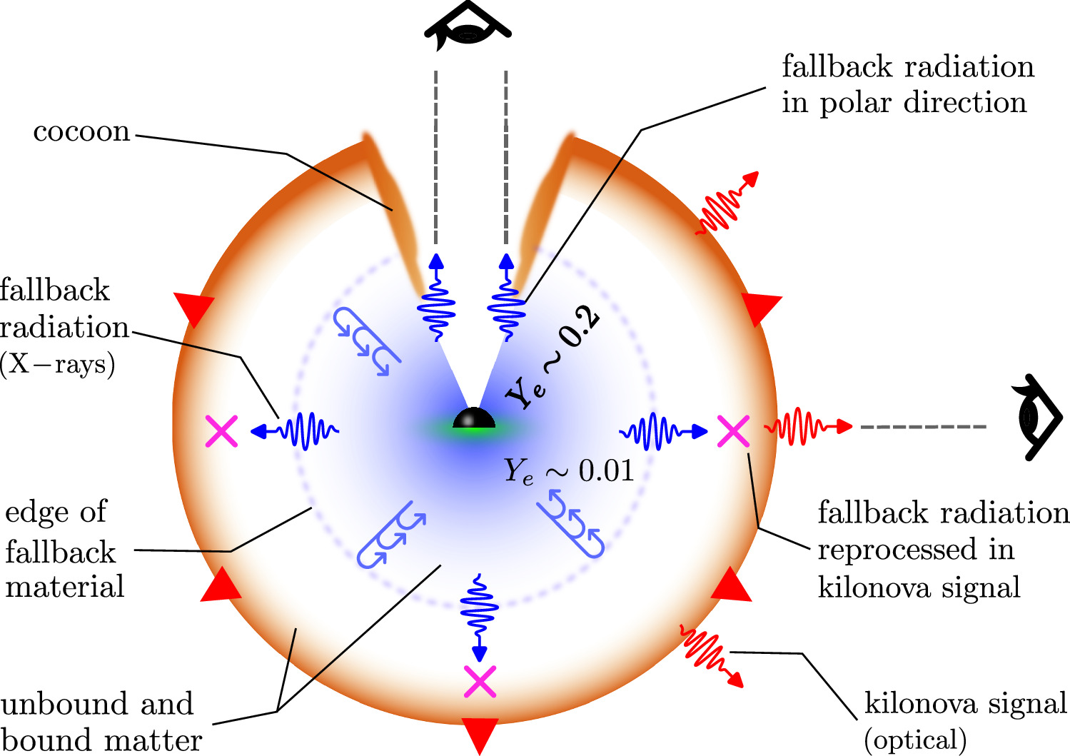