

Abstract
Earth-based gravitational waves interferometric detectors are shot-noise limited in the high-frequency region of their sensitivity band. While enhancing the laser input power is the natural solution to improve on the shot noise limit, higher power also increases the optical aberration budget due to the laser absorption in the highly reflective coatings of mirrors, resulting in a drop of the sensitivity of the detector. Advanced Virgo exploits Hartmann Wavefront Sensors (HWSs) to locally measure the absorption-induced optical aberrations by monitoring the optical path length change in the core optics. Despite the very high sensitivity of Hartmann sensors, temperature fluctuations can cause a spurious curvature term to appear in the reconstructed wavefront due to the thermal expansion of the Hartmann plate, that could affect the accuracy of the aberration monitoring. We present the implementation and validation of a control loop to stabilize the Advanced Virgo HWS temperature at the order of  K, keeping the spurious curvature within the detector's requirements on wavefront sensing accuracy.
Export citation and abstract BibTeX RIS

Original content from this work may be used under the terms of the Creative Commons Attribution 4.0 license. Any further distribution of this work must maintain attribution to the author(s) and the title of the work, journal citation and DOI.
1. Introduction
The dominant noise in the high-frequency region of the sensitivity band of ground-based interferometric gravitational waves detectors is the shot noise limit [1–3] due to Poisson's statistics of photon counting. Although the signal-to-noise ratio of photon counting can be directly improved by increasing the laser input power, this approach has the drawback of enhancing also the amount of laser power absorbed in the substrate and in the coating of the mirrors [4]. The resulting localized heating manifests itself as an inhomogeneous optical path length (OPL) increase originated by non-zero thermo-optic ( ) and thermal expansion (α) coupling coefficients—the so-called thermo-optic effect and thermo-elastic deformation [5], respectively. These power-dependent optical aberrations prevent the detector operating at design sensitivity. Even more impactfully, light scattered from the fundamental mode to higher-order ones makes the error signals for recycling cavity (RC) locking fainter, resulting in a loss of robustness that heavily threatens the detector functionality [5]. In order to monitor the status of power-induced optical aberrations, Advanced Virgo features an array of differential Hartmann Wavefront Sensors (HWSs) looking at the local OPL change in reflection and transmission for all the core optics—i.e. the Input and the End mirrors of the Fabry–Pérot arm cavities [6, 7]. In this class of phase detectors, the beam's wavefront gradient change is measured from the displacement of a pattern of spots projected by a matrix of tiny holes punched in a thin invar-a nickel-iron alloy-plate. The accuracy of the measured optical aberrations is related to the stability of the HWS temperature, since thermal expansion or contraction of the plate contributes to a spurious curvature to the reconstructed wavefront—the so-called thermal defocus. In the following sections, the implementation and validation of a loop for controlling the Advanced Virgo HWS temperature are presented and discussed in detail. The aim of the control loop is to reduce the amount of thermal defocus seen by the HWS well below the wavefront sensitivity requirements set by the Advanced Virgo design [8].
2. Optical aberration sensing: HWS
The HWS currently used in Advanced Virgo have been developed at the University of Adelaide [9] and characterized in the Virgo Tor Vergata laboratories [6, 10]. It is a differential sensor that uses a probe beam reflected from or transmitted through an optical element to locally monitor OPL variations with respect to a reference condition. The probe beam collects a budget of wavefront distortions by interacting with the optical element under test. The distorted beam is then sent to the HWS where it passes through a thin opaque plate containing a matrix of holes-the Hartmann plate (HP)-resulting then in a collection of spots recorded by a charge coupled device (CCD) placed beneath the HP at a fixed distance L referred to as the lever arm. A drawing of a typical HWS setup is shown in figure 1.
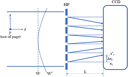
Figure 1. Working principle of the HWS. W and xi
are the reference wavefront and the related position of the ith spot resulting from it, respectively, while W and
and  refer to a generic wavefront acquired during the measurement. Reproduced with permission from [9].
Download figure:
Standard image High-resolution imageConsider a beam with wavefront W affected by optical aberrations passing through the HP and producing a set of spots recorded by the CCD. Then, the position
  of the ith spot is determined by a centroid identification algorithm and the displacement Δxi
of each spot from a previously measured reference position xi
is evaluated. Finally, the data set of all the centroid measurements provides the gradient of the wavefront as [9, 11]:
of the ith spot is determined by a centroid identification algorithm and the displacement Δxi
of each spot from a previously measured reference position xi
is evaluated. Finally, the data set of all the centroid measurements provides the gradient of the wavefront as [9, 11]:

with the wavefront change ΔW computed by numerically integrating the discrete gradient field.
The HWS probe beam is produced by a superluminescent emitting diode (SLED), i.e. a broadband source characterized by a short coherence length that eliminates interference between stray beams.
In order to minimize the thermo-elastic deformation, the 50 µm thick HP is made of invar. HP's holes have a diameter of 150 µm and they are arranged in a hexagonal pattern, spaced 430 µm apart from each other. The plate is supported by a 3 mm thick invar spacer in front of the CCD-with a nominal lever arm of 10 mm-and it is kept in position by a 3 mm thick invar cover slab and protected by a transparent window [9]. The hole diameter, pitch, pattern and value of L were optimized to ensure that cross-talk between neighbouring spots was negligible while maintaining sensitivity [12]. The CCD is composed by  pixels, with an active area of
  cm and a maximum acquisition rate of 60 frame per second [13]. As supplied by the manufacturer, the CCD is housed within an aluminum case.
The heat produced by the CCD operation is transferred through two slabs of copper towards dissipating fins. In order to improve the heat conduction between the CCD and the fins, a little layer of Sil-Pad 1500ST—a thermocondutive silicon-based material—is placed between the CCD and the copper slabs and between the copper slabs and the fins as well. A schematic view of the HWS assembly with all its components is shown in figure 2.
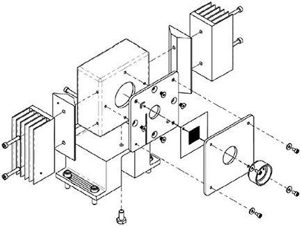
Figure 2. A view of the assembly [14] of the HWS currently in operation in the Advanced Virgo detector. Reproduced from [14]. CC BY 4.0.
Download figure:
Standard image High-resolution imageTwo different setups have been installed in Advanced Virgo to monitor the local OPL change upon reflection from and transmission through the core optics [6, 15]. Two HWSs measure the thermal lens 5 on the two input mirrors crossed by the laser beam—the so-called HWS in transmission, or on-axis setup—while four wavefront sensing setups—HWSs in reflection, or off-axis setup—have been designed to measure the thermoelastic deformation 6 on the input and end mirrors. The two HWSs in transmission and their probe beam SLEDs are hosted on the Injection and Detection areas to sense the thermal lenses on the input mirrors—West Input and North Input, respectively. The HWS in reflection are hosted on an in-air optical optical bench installed outside of the mirrors' vacuum chamber [16]. The key feature of both layouts is that the HWS is placed in the image plane of the monitored optic, so to directly rescale the wavefront distortion seen by the HWS to the plane where the distortion is induced. A simplified scheme of the setups is shown in figure 3.
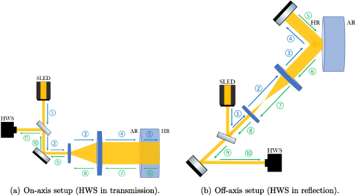
Figure 3. Outline of the setups for the evaluation of the absorption-induced OPL change. The on-axis measurements—figure (a)—are carried on by the HWSs in transmission to monitor the thermal lens effect in the Input mirrors of the Fabry–Pérot arm cavities. The off-axis measurements—figure (b)—are taken by the HWSs in reflection to detect the thermoelastic deformation in both Input and End mirrors of the Fabry-Pérot arm cavities. The yellow beam represents the probe beam (SLED), while the blue and the green arrows and numbers highlight the onward and the reflected beam in the light path, respectively. The AR and HR indicate the anti-reflective and the high-reflective side of the optical element, respectively. In order to sense the aberrations in a wide area around the optical axis, an afocal telescope is used to increase the size of the probe beam on the mirror surface.
Download figure:
Standard image High-resolution image2.1. Thermal defocus
The thermal expansion or contraction of the HWS components due to environmental temperature fluctuations affects the HWS performance, resulting in the generation of a spurious curvature in the reconstructed wavefront. Spurious contributions to the wavefront curvature coupled to temperature variations are usually termed as thermal defocus [6]. In order to estimate it, we must precisely know the response of the HWS components' materials to a temperature variation—which is quantified by their thermal expansion coefficient α.
We can identify two main effects which can contribute to thermal defocus: thermal expansion/contraction of the HP and thermal expansion/contraction of the CCD. Both of them result in an increase/decrease in the distance between the holes and, therefore, between the CCD spots which, in turn, changes the wavefront gradient measured by the sensor. Because the CCD sensor is a metal-oxide-semiconductor [13], it is expected to expand/contract less than the HP—which is made of invar. Therefore, the effect of the CCD surface deformation is henceforth neglected.
To compute the thermal defocus, we consider a beam ray having divergence angle θ and radius of curvature RoC. The beam ray propagates through a HP hole and after traveling the distance  —where the radius of curvature becomes RoC
 —it impinges on the CCD as shown in figure 4.
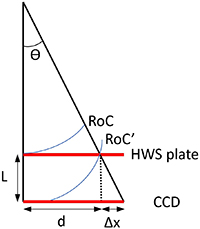
Figure 4. Sketch of the propagation of a beam ray in the HWS at a fixed temperature. After passing through a HP hole, the ray impinges on the CCD at a distance d from the centre. Here the displayed change in the RoC is due only to the beam propagation and not to thermal effects.
Download figure:
Standard image High-resolution imageFor small values of θ, we can assume RoC  RoC
RoC and
and  . The spot displacement Δx on the CCD with respect to a reference plane wave is related to the radius of curvature of the wavefront by

where d is the distance between the optical axis and the HP hole as displayed in figure 4.
The HP thermal expansion/contraction generates a transversal displacement of the hole, resulting in a variation Δd of the projection of the hole on the CCD surface and in a change Δθ of the divergence as well [6]. Moreover, also a variation ΔL of the distance between the HP and the CCD can provide a non-negligible contribution to the spot displacement on the CCD, as it is visible from figure 5.
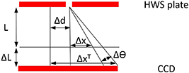
Figure 5. Effects of the thermal expansion on the final position of the beam impinging on the CCD. The displacement of the plate hole changes θ and d of an amount Δθ and Δd, respectively, while the lever arm increases by ΔL. The combination of all these effects changes the spot displacement on the CCD from Δx to ΔxT —see equation (3).
Download figure:
Standard image High-resolution imageTaking into account all these effects, the total displacement ΔxT of the spot on the CCD can therefore be evaluated as

with  . The thermal variations for d and L due to a small temperature fluctuation ΔT are given by


where αd and αL are the linear thermal expansion coefficient for d and L, respectively. For small temperature changes, we can retain only the first-order terms in equation (3). Therefore, combining equations (3), (4a ) and (4b ) and assmuning θ and ΔT to be small, we can rewrite the displacement ΔxT as

where the first term is the displacement Δx given by equation (2).
Finally, if RoC  L, it is possible to rewrite equation (5) as

from which it emerges that the most relevant effect of the HWS thermal expansion is on Δd, i.e. on the distance between two adjacent holes of the HP.
By imposing  in equation (6), the wavefront RoC for which the curvature one would observe is equal and opposite to the spurious contribution due to the thermal expansion can be computed—this is the so-called critical RoC

which, rewritten in terms of curvature, gives the spurious curvature C due to the thermal defocus that is measured by the HWS and its direct relation with the HWS temperature fluctuations ΔT, i.e.

2.2. Advanced Virgo requirements
The impact of local aberrations in Advanced Virgo operation has been extensively characterized in relation to the design [8]. These studies provided a set of requirements in terms of OPL residual distortion in the RC and core optics surface RoC accuracy, which is summarized in table 1 [8].
Table 1. Advanced Virgo general requirements on wavefront distortion.
| Parameter | Requirement |
|---|---|
| RC residual OPL RMS |
 2 nm 2 nm |
| Core optics RoC precision | ±2 m |
The sensitivity of HWSs must be at least one order of magnitude better than the requirements in terms of OPL variation. This implies an additional requirement on the maximum allowable HP temperature swing, in order to keep the thermal defocus well below the required sensitivity.
2.2.1. Temperature stabilization for the RC residual OPL requirement.
The limit to the HWS thermal defocus can be computed starting from the requirement ΔW = 2 nm RMS. In the computation, we must consider—besides the requirement on the HWS sensitivity to be at least one order of magnitude better than the requirements in terms of OPL variation—also an additional factor of two due to the double-pass configuration in which the HWS operates [4]—which would give an RMS limit of 0.4 nm. While the requirement is expressed in terms of the wavefront RMS, it is simpler to put a constraint on the maximum amplitude of the thermal defocus term. It can be shown that the RMS value of a spherical wavefront over an aperture is smaller than its maximum amplitude by a factor 2 . So, in order to translate the RMS into a limit on the amplitude of the defocus term, we must multiply it by a factor 2
 , ending with a defocus limit of 1.39 nm RMS. Therefore, the maximum allowable wavefront variation
  due to the temperature fluctuation
  can be written from equation (8) as

where D is the dimension of the CCD sensitive area. Rearranging equation (9) in order to constrain  , assuming
  K−1—that is a reasonable choice for a generic invar [17]—and D = 12.28 mm for the CCD, the maximum allowed temperature fluctuation
  results to be

2.2.2. Temperature stabilization for the TM RoC precision requirement.
An additional requirement is related to the required accuracy of ±2 m in the tuning of the core optics RoC. A wavefront reflected back by a mirror surface with a given RoC accumulates a curvature C given by

since reflection is intrinsically a double-pass process. If the RoC deviates from its nominal value by a small quantity  RoC, the corresponding variation in curvature is

In order to derive the curvature variation measured by the HWS, we should include in equation (12) the square of the telescope magnification factor M and an additional factor of two because of the double-pass measurement scheme in the off-axis layout [6], which gives

As for the previous section, in order to compute the maximum permissible temperature variation  we impose a measurement accuracy one order of magnitude better than the requirement, which results in

Using equations (8) and (14), M = 7, RoC = 1500 m, ε = 2 m and assuming again  K−1, the maximum temperature variation can be computed as

which results to be the most stringent sensing requirement.
3. Temperature stabilization
The temperature swing limits computed in the previous section cannot be guaranteed by the air-conditioning system of the Advanced Virgo infrastructure [10]. Therefore, an active control system that maintains the HWS temperature within the requirement in equation (15) is necessary. Moreover, since the thermal phenomena—thermal lensing and thermoeleastic deformation—responsible for the aberrations measured and monitored by the HWS have a characteristic time of many hours, the HWS temperature stability must hold for time intervals of the order of the day.
The development and characterization of the temperature stabilization control has been carried on in a dedicated facility— Testing TCS integrated strategies (TeTis) [6]—in the Virgo Tor Vergata laboratories.
3.1. CCD, sensors and actuators
The HWS CCD case is installed on an aluminum support—mounted on the optical bench of TeTis—in order to dissipate the heat produced when it is switched on. As it will be described later, the base can be either a simple post or a larger custom-made support.
In order to monitor the CCD temperature, PT100 [18] resistance temperature detectors (RTDs) have been used. Two PT100 sensors have been placed on the left and on the bottom of the sensor front invar cover, respectively. They have been labeled as the Witness and the Controller, respectively, with the former (out-of-loop sensor) measuring the actual temperature of the invar cover, while the latter is in-loop with the control system actuators. An additional PT100 is anchored to the optical bench to measure environmental temperature fluctuations. To stabilize the CCD temperature within the requirements, an actuator capable of subtracting and/or supplying the right amount of heat is needed. The selected actuator is a thermoelectric Peltier cell, which operates exploiting the Peltier effect [19, 20].
3.2. Loop implementation and temperature stabilization results
In order to properly control the temperature fluctuations of the HWS, a proportional-integrative-derivative (PID) control loop has been designed and implemented. The output u(t) of this control can be written as [21]

where  ,
,  and
and  are the proportional, integral and derivative gain, respectively, and e(t) is the error signal defined as the difference between the chosen setpoint and the process variable. The output u(t) can be rewritten as a function of the integral and derivative time
  and
and  , respectively, as

Using the Ziegler–Nichols method [22], a preliminary estimation of the PID parameters has been computed. The control loop has been then tested with the Ziegler–Nichols settings and subsequently fine-tuned by changing the PID parameters until the best performance in terms of temperature stability has been reached. The final optimized PID parameters and the comparison with the Ziegler–Nichols settings are summarised in table 2.
Table 2. Optimized parameters for the HWS temperature control system compared with the ones computed with the Ziegler-Nichols method.
| Parameter | Ziegler–Nichols | Optimized |
|---|---|---|

| 3 | 8 |

| 10 min | 2.5 min |

| 0.27 min | 2 min |
| Sampling time | — | 10 s |
| Number of averages | — | 6 |
Using these optimal settings, the control loop has been tested with the HWS in three different configurations:
- Configuration A: the HWS is mounted on an aluminum cylindrical post, with the Peltier cells placed between the copper layer and the fins.
- Configuration B: the HWS is mounted on a bulky support made of aluminum, while the Peltier cells are left in the same position as in the previous configuration.
- Configuration C: the HWS is mounted on the same support as in the previous configuration, but in order to try to reduce the dependence of the HWS temperature from the fluctuations of the environment, the Peltier cells have been placed below the HWS—i.e. between it and the aluminum support.
The whole assembly of the HWS in all the three configurations with the PT100 RTDs mechanically anchored on the front cover and the two Peltier cells is shown in figure 6.
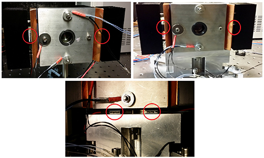
Figure 6. The HWS installed in TeTis in Configuration A (top left), B (top right) and C (bottom), respectively. The position of the Peltier cells in the different Configurations is marked with a circle. In all the Configurations two Peltier cells were used, although in the figure for A and B the cell on the right hand side of the HWS in not visible. In A, an additional PT1000 witness RTD was used in the preliminary tests and lately removed.
Download figure:
Standard image High-resolution imageThe efficiency and the stability of the control loop were tested on timescales from few hours to week-long measurements. In all cases, the control is able to provide a temperature stabilization  0.01 K and to maintain it on long timescale, compensating for the day/night temperature variations. An example of the provided stability is shown in figures 7 and 8, while the typical results obtained for each configuration are summarized in table 3.
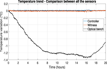
Figure 7. Typical temperature variations on the HWS compared to the trend of the environmental temperature as measured by the RTD on the bench.
Download figure:
Standard image High-resolution image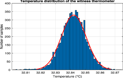
Figure 8. Temperature distribution of the PT100 witness (out-of-loop) thermometer in configuration C. In this measurement the temperature was controlled to a mean value of 32.8422 ∘C within a fluctuation of 0.0078 ∘C.
Download figure:
Standard image High-resolution imageTable 3. Typical results obtained in terms of temperature stability in all the tested configurations, expressed as standard deviation values for both the PT100 sensors.
| Configuration |

|

| Duration |
|---|---|---|---|
| A | 0.0088 ∘C | 0.0095 ∘C | 22 h and 23 min |
| B | 0.0044 ∘C | 0.0051 ∘C | 114 h and 55 min |
| C | 0.0072 ∘C | 0.0078 ∘C | 22 h and 45 min |
4. Thermal defocus measurements
In the Advanced Virgo design configurations (figure 3), the SLED source is collimated and expanded using dedicated optics. However, these optical systems can cause additional thermal defocus due to the thermal expansion of their supporting structures. Since we are only interested in characterizing the defocus originated by the HP, no optics have been installed between the SLED and the sensor. The optimal size [9] of the beam on the sensor was obtained by putting the HWS at 11 cm from the SLED source and exploiting the natural divergence of the SLED beam. The lever arm of the particular HWS used for this study was measured as L = 9 mm.
In order to estimate the wavefront curvature to be compared with the defocus formula in equation (8) for any chosen setpoint of the temperature control, a frameset of 100 wavefront maps was reconstructed by numerically integrating the local gradient fields measured by the HWS. The wavefronts in the set are averaged to get rid of noise. Any of the averaged wavefronts, corresponding to a specific HWS temperature, is referred to the first acquired wavefront as a reference. The curvature term is then extracted by fitting the wavefront with a second-order model over the HP aperture.
As detailed in the next section, the wavefront measurements were performed in two different experimental configurations (shown in figure 9) :
- Vertical setup: the HP is installed in vertical position and the SLED beam propagates parallel to the optical bench.
- Horizontal setup: the HP is horizontal and the optical axis is perpendicular to the bench, with the SLED source in position above the HWS.
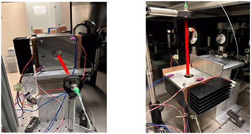
Figure 9. Vertical (left) and horizontal (right) experimental setups. The light source is placed at a distance of about 11 cm from the HP. The red beam has been drawn to highlight the system optical axis. In the horizontal setup, the witness and controller sensors are both glued on the spacer.
Download figure:
Standard image High-resolution image4.1. Vertical setup
The measurements are aimed at highlighting the expected correlation between the curvature of the observed wavefronts and the HWS temperature variation when changing the setpoint of the control loop. The measured curvature in two different measurements is compared in figure 10 with the nominal value predicted by equation (8) assuming a free standing invar HP, that is, a value of  K−1. The correlation is clearly evident, confirming that the observed curvature is indeed a thermal defocus. However, with this choice of αd
, the measured curvature does not match the expected one.
K−1. The correlation is clearly evident, confirming that the observed curvature is indeed a thermal defocus. However, with this choice of αd
, the measured curvature does not match the expected one.
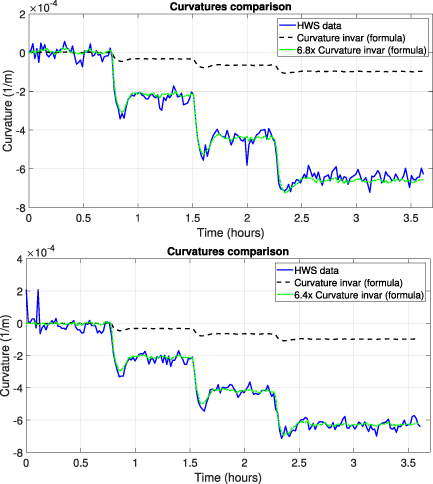
Figure 10. The wavefronts curvature obtained from vertical setup measurements compared to the spurious curvature due to the thermal expansion of the HP invar plate. In order to match them, it was necessary to multiply the invar curvature by a factor 6.8 (top measurement) or 6.4 (bottom measurement), respectively.
Download figure:
Standard image High-resolution imageTo recover an optimal matching, it is necessary to multiply the nominal curvature by an effective factor k estimated, in a least-squares sense, by finding the value that minimizes the χ2

where  is the number of wavefront acquired during a measurement,
  are the measured curvature values and
  are the theoretical ones. In order to quantify the best estimate and the uncertainty associated with this definition of the factor k, a statistical analysis has been applied. Curvature measurements taken in the same conditions can be regarded as a set of measurements of a random variable with Gaussian distribution. Therefore, for each temperature step the curvature mean value was computed with the relative standard deviation

where  is the standard deviation for the ith step and Ni
is the total number of curvature samples in that step. These values as a function of the relevant
is the standard deviation for the ith step and Ni
is the total number of curvature samples in that step. These values as a function of the relevant  have been fitted with a function
  using the least-squares method, as shown in figure 11.
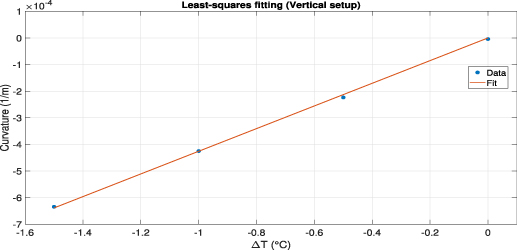
Figure 11. The measured curvature trend as a function of the witness sensor ΔT. The interpolated linear fit is also shown.
Download figure:
Standard image High-resolution imageThe resulting slope of the fit is B = 4.26 · 10−4 K−1 m−1 and the uncertainty on this value is σB = 2.69 · 10−6 K−1 m−1. The coefficient B is related to the thermal expansion coefficient α by equation (8)

Considering the obtained value for B with its uncertainty and a lever arm of L = ( ) mm, the measured curvature is compatible with an effective thermal expansion coefficient equal to
  K−1. Thus, the ratio between the experimental value of α and the expected one, expressed by the previously-defined factor k, is given by

4.2. Horizontal setup
A possible explanation of the observed value k > 1 is the presence of a coupled thermal expansion between the CCD aluminum case and the invar components (HP, spacer, front plate) that are mechanically constrained to the case by four screws. Since the aluminum has an expansion coefficient one order of magnitude higher than that of the invar, the HP and the plates are expected to be dragged by the CCD case deformation. In order to investigate the hypothesis, the HWS was installed in the horizontal configuration shown in figure 9. In this way, it was possible to loosen the screws and then to mechanically disentangle the CCD case from the HP. In order to maintain a good thermal contact between the RTDs and the invar front plate, the PT100s were glued on the plate through a conductive paste—this ensured a good control loop stability.
As for the vertical setup measurements, the setpoint of the control loop was changed a few times during the wavefront acquisition. Noticeably, in this configuration the discrepancy between the expected and experimentally measured curvature values was lower with respect to the previous set of measurements, as shown in figure 12 in two different measurements.
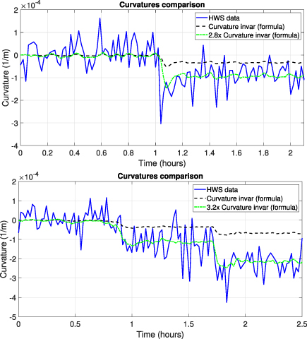
Figure 12. The wavefronts curvature obtained in the horizontal setup measurements compared to the spurious curvature due to the thermal expansion of the HP invar plate. In order to match them, also in this configuration it was necessary to multiply the invar curvature by a factor 2.8 (top measurement) or 3.2 (bottom measurement), respectively.
Download figure:
Standard image High-resolution imageSince all the data collections were carried out in almost the same experimental conditions, the same statistical analysis used for the vertical setup measurements was performed in order to assess the best estimate of the k factor. The resulting least-squares fitting is shown in figure 13.
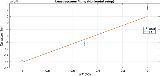
Figure 13. The measured curvature trend as a function of the witness sensor ΔT. The interpolated linear fit is also shown.
Download figure:
Standard image High-resolution imageFor this experimental setup, the slope of the fit is B =  K−1 m−1 and the related uncertainty on this value σB
= 0.42 · 10−6 K−1 m−1. The obtained effective thermal expansion coefficient is
K−1 m−1 and the related uncertainty on this value σB
= 0.42 · 10−6 K−1 m−1. The obtained effective thermal expansion coefficient is  K−1. Therefore, the ratio between the effective value of α and the expected one is

4.3. Results
Moving from the vertical configuration—the one in which the HWSs are currently mounted in Advanced Virgo—to the horizontal one, the discrepancy between the measured curvature and the thermal defocus obtained by assuming a nominal value of  K−1 was actually reduced, as demonstrated by the drop of the matching factor from k ∼ 6 down to k ∼ 2. This reduction confirms the hypothesis of a coupling between the invar components and the CCD case.
We therefore assume that, in the measurements with the horizontal setup, the HP was efficiently decoupled from the CCD case. In this case, the estimated thermal expansion coefficient is  K−1. Assuming that the invar type of the HP is the most common one—the so-called invar 36 containing 64
 of Iron and 36
 of Nickel [23–26]—the thermal expansion coefficient is expected to be in the range [0.5–2.0] · 10−6 K−1. Given the associated uncertainty in the final computed αd
, the obtained values are compatible with this range.
of Nickel [23–26]—the thermal expansion coefficient is expected to be in the range [0.5–2.0] · 10−6 K−1. Given the associated uncertainty in the final computed αd
, the obtained values are compatible with this range.
The maximum allowed temperature swing can be recalculated from the coefficients obtained in the two different configurations by using equations (10) and (15) as constrained by the Advanced Virgo requirements. Since the measured expansion coefficients are larger than the assumed value for αd , the final requirements on the maximum allowed temperature fluctuation are tighter—see table 4.
Table 4. The maximum allowed temperature fluctuation  as constrained by the Advanced Virgo requirements, computed from the experimentally measured linear thermal expansion coefficients.
| Configuration | αd (10−6 K−1) |
 (K) (K) |
|---|---|---|
| Vertical | 7.7±0.9 | 0.02 |
| Horizontal | 2.6±1.0 | 0.05 |
5. Conclusions
A proper monitoring of the optical aberrations budget in Advanced Virgo requires the Hartmann sensors to be temperature-stabilized at the order of few hundredths of degree. For this purpose, a PID control loop was designed, implemented and tested, resulting to be able to provide a temperature stabilization within the requirements. The thermal defocus measurements—performed in two different experimental configurations—provided evidence that a higher-than-expected effective thermal expansion coefficient α is due to a coupling of the thermal expansion of the invar components with that of the aluminum CCD housing.
Given the measured α in the vertical configuration—the one currently implemented in Advanced Virgo—the maximum permissible temperature fluctuation is  K. This is slightly larger than the deviation value obtained by stabilizing the HWS temperature with the designed PID control system, which can assure a temperature stabilization at the order of
  K.
K.
In order to further reduce the thermal defocus contribution, different upgrades can be developed and/or adopted in the future. For example, refined filters can be designed and tested to have a better control loop response. Larger Peltier cells can be exploited, resulting in wider dynamics of the control. At the same time, in the design of the new HWS planned for the next upgrades of Advanced Virgo, the CCD case will be realized in invar in order to be intrinsically less sensitive to environmental temperature variations—which are expected to be lower in the future, by exploiting a better control of the environmental temperature in Advanced Virgo experimental areas.
Acknowledgments
The authors thank R Simonetti and A Bazzichi for their precious technical assistance. L A thanks his previous affiliation (Gravity Exploration Institute, Cardiff University) for supporting him to work on this paper. This work was promoted by the Virgo Collaboration and supported by INFN Roma Tor Vergata and University of Roma Tor Vergata.
Data availability statement
All data that support the findings of this study are included within the article (and any supplementary files).
Footnotes
- 5
This effect is due to the dependence of the refractive index from temperature
 . The power absorbed in the substrate and in the coating generates a temperature gradient inside the optics and so its refractive index changes from the nominal one generating the so-called thermal lensing.
 - 6
This is due to the non-zero thermal expansion coefficient α, with the consequence that the surface of an heated optic expands along the optical axis and induces a change of the Radius of Curvature of the mirror from the nominal one.
