Study on ice resistance of Antarctic krill ship with trawl under floating ice sea conditions

1 Introduction

The Antarctic krill, scientifically known as Euphausia superba, is a keystone species in the Southern Ocean ecosystem. It is also regarded as the largest single catchable biological resource in oceans worldwide (Rod et al., 2022). The distribution of Antarctic krill follows a circum-Antarctic distribution pattern, usually located in waters south of 50°S. These include the waters off the Antarctic Peninsula, the Antarctic continental shelf edge and the Southeast Antarctic Ocean. Popular areas currently being exploited include Vilkes Bay (68°S, 78°W), Bourbosse Strait (63°S, 57°W), the Ross Sea (160° to 180°W, 70° to 78°S), and the Amundsen Sea (90° to 150°W, 65° to 75°S). Figure 1 illustrates the extent of krill distribution in Antarctic waters, with the yellow areas showing the areas where CCAMLR catch limits apply (Yang et al., 2020). The density of ice flow distribution varies seasonally and latitudinally, and the sea area covered in this study ranges from 60° to 80°S.

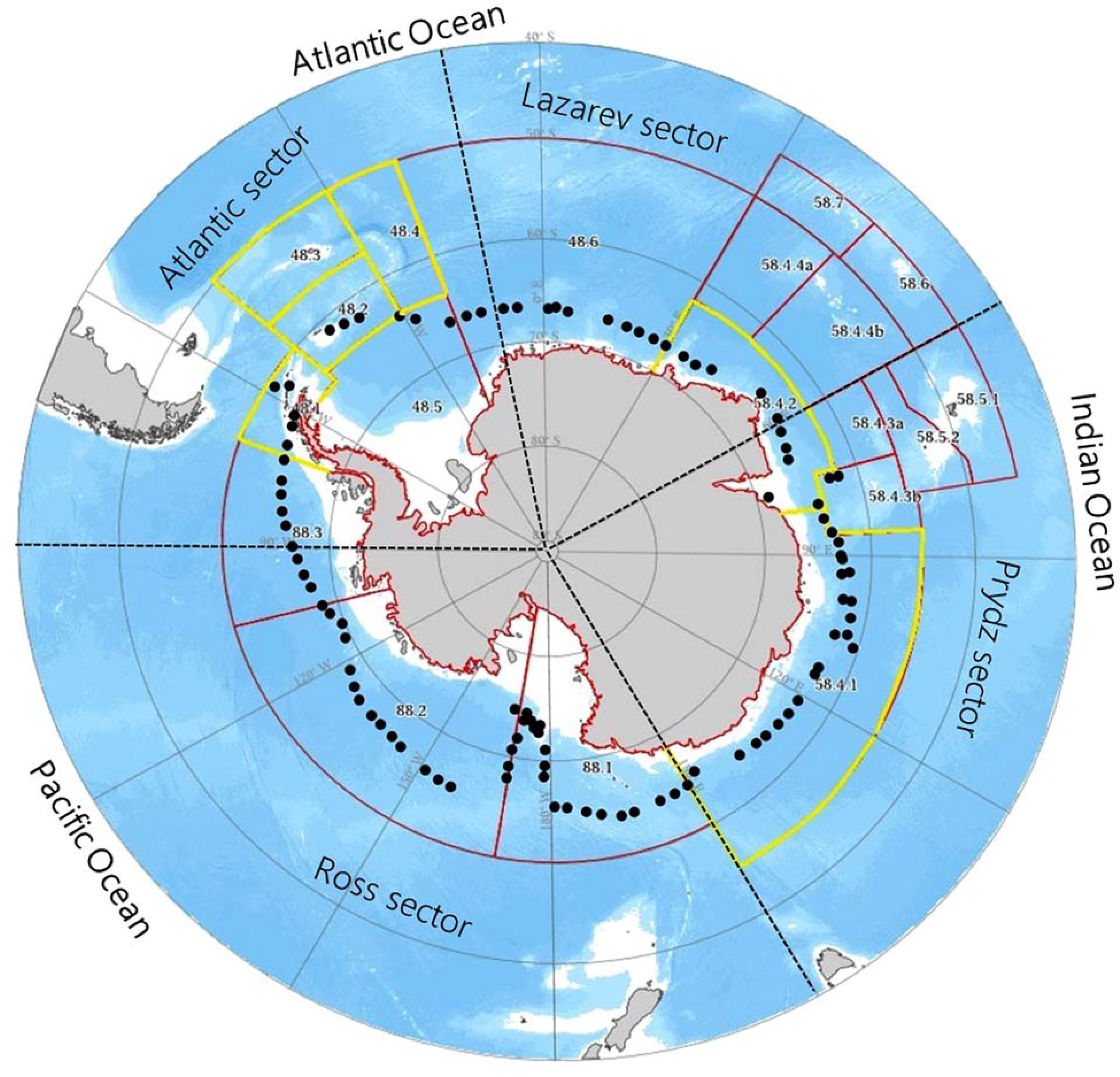
Figure 1 Extent of Antarctic waters and distribution of krill.

The Antarctic krill contains a high concentration of endogenous hydrolase, which is readily autolytic, thereby resulting in a rapid decline in its freshness with time. Consequently, there is a high demand placed on vessels and equipment for Antarctic krill fishing (Patricio et al., 2016). Professional fishing and processing vessels with advanced technology serve as a powerful and necessary tool for Antarctic krill fisheries (Wang et al., 2021). These vessels operate in the Antarctic Sea area and frequently interact with ice flows while sailing or operating. This interaction between the vessels and ice flows is a complex process, which is more dangerous in Antarctic waters (Huang et al., 2016).

The primary distinction between Antarctic waters and other waters is the prevalence of drift ice. As a consequence of global warming, ice flow fields are anticipated to become the most prevalent environment for polar transport (Thomson et al., 2018; Chen et al., 2021; Sun et al., 2022). Consequently, a number of experiments have been conducted to examine the capability of fishing vessels to navigate through ice (Kim et al., 2014, Kim et al., 2019; Cai et al., 2022; Xie et al., 2023). The results of these experiments indicate that ice flows may have a substantial effect on such vessels, which emphasises the importance of predicting ice resistance. Consequently, during the vessel design phase, it is of paramount importance to accurately assess the ice-going capability of the vessel. Shipyards must determine the most effective and economical propulsion capacity and hull shape (Zhong et al., 2023).

Only a few studies have investigated the resistance of ships sailing in broken ice through experimental methods (Kim et al., 2013; Guo et al., 2018a; Huang et al., 2022). Given the considerable time and cost requirements associated with experimental testing, empirical formulas can serve as a supplement to model tests for estimating the ice resistance of ships during the early design stage. A plethora of empirical formulas have been developed to calculate ice resistance under various ice conditions (Lewis et al., 1982; Erceg and Ehlers, 2017; Koto and Afrizal, 2017). However, these semiempirical models have been specifically designed for particular types of ships or even specific ice conditions, which potentially leads to estimation errors when formulas are used inappropriately. Consequently, the prediction of ship drag in the presence of diverse ice flows remains a challenging task (Zong and Zhou, 2019).

In recent years, researchers have used numerical simulation techniques to investigate the interaction between ice and structures. For instance, Coetzee (2016) used a combination of theoretical analysis and experimental techniques to establish the discrete-element method (DEM) standards, select appropriate parameters and evaluate the effect of particle shape. Jiménez-Herrera et al (2018) used commercial DEM calculation software to examine the fragmentation model of DEM particles under the impact, analyze and compare three types of failure models, and provide guidance for enhancing and optimizing the internal failure model of DEM particles. Various numerical methods have been used to simulate ice damage, including the finite-element method (Guo et al., 2018b; Tan et al., 2013), the DEM (Lau et al., 2011; Polojärvi and Tuhkuri, 2013), peridynamics (Zhao, 2016; Lu, 2018), and smoothed particle hydrodynamics (Gutfraind and Savage, 1998; Shen et al., 2000; Das, 2017). Among these methods, the DEM has been used to model the geometric and physical state of ice flows (which can clearly demonstrate changes in stress, displacement, and velocity) and study the motion and ice load experienced by ships sailing in ice flow areas (Lau et al., 2011; Dai et al., 2022).

The major difference between Antarctic krill vessels and general vessels is that Antarctic krill trawls stretch out during fishing. Currently, research on Antarctic krill trawls primarily focuses on net shape (Zhu et al., 2023) and the effect of simulated catches on nets (Cheng et al., 2022). Only a few studies have examined the ice resistance of Antarctic krill vessels. In the present study, an Antarctic krill ship with a length of 120m was used as the object for the study. Given the characteristics of Antarctic krill ships navigating and trawling through ice flow areas, the CFD-DEM method is applied to simulate the navigation of the Antarctic krill ship in an ice flow and the numerical simulation was conducted by the commercial software STAR-CCM+ (Siemens Digital Industries Software, Plano, TX, USA). The verification and validation of the numerical method were conducted by results of the tank test first. Then, the total resistance and drag characteristics of the Antarctic krill ship while navigating through a floating-ice area were evaluated (Guan et al., 2022; Tang et al., 2022).

This study is concerned with the drag characteristics of a Chinese Antarctic krill ship employing a continuous pumping fishing technique in an ice flow area. The first half of section 2 describes the ship-ice interaction model and the fluid-solid coupling model used in this study. The second half of the section details the parameters of the Antarctic krill ship and trawl. Section 3’s first half describes the ice drag calculation based on the STAR CCM+ software and a comparison with the model experiments. The second half compares the effects of ice flow density and speed on the ship’s navigational resistance. The information obtained is analysed and discussed in Section 4. Finally, the conclusions of this paper are drawn. This paper provides a reference for improving the ship’s wave resistance and fishing ability.

2 Materials and methods

2.1 Basic equation

The CFD-DEM method was used to analyse the interaction between ship and floating ice. In general, ice flows should constantly satisfy Newton’s second law of motion (Norouzi et al., 2016; Georgiev and Garbatov, 2021). The following are the equations of motion under the actions of force and moment:

In Equations (1) and (2), v_i is the speed of floating ice i, F_ij is the noncontact force between floating ice i and floating ice j or other pieces of floating ice, F_g is the weight of the floating ice, F_fluid is the fluid force, I_i is the rotational inertia of floating ice i, ω_i is the angular velocity of floating ice i, and T_ij is the contact moment acting on floating ice i because of a contact force other than floating-ice gravity.

2.2 Contact force

In STAR-CCM+, a spring–damper system is used to calculate the contact force. In this calculation, overlaps between the particles and the wall are allowed, and an elastic force is generated by the spring. The contact force between the particles is represented as follows:

In Equation (3) F_n is the normal force of contact between two floating-ice particles and F_t is the tangential force of contact between these particles.

A linear spring–damper contact model is used as the contact model in this study. The following equations express the normal component F_n and tangential component F_t of the contact force F_contact:

In Equations (4) and (5) k is the modulus of elasticity; η represents damping, which is the energy consumed by the contact between particles; d_n and d_t are the overlap distances in the normal and tangential directions, respectively; V_n and V_t are the normal and tangential components, respectively, of the relative velocity between two contact particles; C_f is the friction coefficient, which is set as 0.35 between ice particles and 0.05 between the hull and ice particles (Han, 2021); k_n is the normal spring stiffness; k_t is the tangential spring stiffness; η_n represents the normal damping; and η_t represents the tangential damping.

In Equations (6) – (8), ηndamp is the normal damping coefficient, ηtdamp is the tangential damping coefficient, M_eq is the equivalent mass of floating-ice particles, and M_A and M_B are the equivalent masses of floating-ice contact particles A and B, respectively.

The contact force between solid ice particles and dry, rigid, and unbreakable hulls is described by the Hertz–Mindlin contact model as follows (Walton, 1987):

In Equations (9) - (13) δ_max is the maximum overlap distance; E_eq is the equivalent Young’s modulus; v_A and v_B are Poisson’s ratios of particles A and B, respectively; E_A and E_B are Young’s moduli of particles A and B, respectively; R_eq is the equivalent radius; R_A and R_B are the radii of particles A and B, respectively; and G_eq is the equivalent shear modulus.

For collisions between particles and walls, the wall radius R_wall can be assumed to be ∞, with the wall mass M_wall being ∞. Consequently, from the aforementioned formulas, the equivalent radius R_eq is equal to R_particle, and the equivalent mass M_eq is equal to M_particle.

2.3 Governing equation of fluid mechanics

According to the continuity equation, the net mass flowing out of a microelement per unit time is equal to the decrease in the mass of the microelement during that time.

In Equation (14), $\nabla$ is a Hamiltonian operator.

The momentum Equations (15) and (16) indicate that the rate of momentum change in the fluid microelement is equal to the rate of change of momentum entering or leaving the surface of the Control volume, plus the sum of various forces acting on the fluid microelement.

In Equation (17), V = (u, v, w) represents the momentum conservation equation in the x-direction, y-direction, and z-direction, respectively; f is the volume force acting on the microelement; τ is the stress tensor; and p is the pressure acting on the microelement.

2.4 Turbulence model

In this study, the standard k–ϵ model was used as the turbulence model. The transport equations for turbulent flow energy k and dissipation rate ϵ are expressed as follows:

In Equations (18) and (19), $G_k=\mu (\frac{\partial {\mu }_i}{\partial x_j}+\frac{\partial {\mu }_j}{\partial x_i})\frac{\partial {\mu }_i}{\partial x_j}$ turbulence viscosity equation, ${\mu }_{\text{t}}=\rho C_{\mu }\frac{{\text{k}}^2}{ϵ}$. Reynolds Shear stress equation $-\rho {{\overline{\text{u}}}^{\prime }}_{\text{i}}{{\overline{\text{u}}}^{\prime }}_{\text{j}}=\mu (\frac{\partial {\overline{\text{u}}}_i}{\partial x_j}+\frac{\partial {\overline{\text{u}}}_j}{\partial x_i})-\frac{2}{3}\rho \text{k}{\delta }_{\text{ij}}$.

2.5 Boundary condition and grid generation

This study focused on a Chinese Antarctic krill vessel operating with continuous pumping fishing technology. Its reference ship is Shenlan Antarctic krill ship, which is the first self-developed Antarctic krill fishing ship in China. It was built by Jiangsu Shenlan Ocean Fishery Co., LTD., a subsidiary of China Shipbuilding Corporation, Huangpu Wenchong Shipping Co., LTD. 708 Institute participated in the design. The Deep Blue Antarctic krill ship is a large ocean-going fishing boat with advanced technology and complete functions, with strong fishing and processing capacity, which provides strong support for the development of China’s Antarctic krill resources. An Antarctic krill ship’s hull and a middle trawl for Antarctic krill, were used in the numerical simulation. The middle trawl had a lower-class length S of 55.68 m, a horizontal spacing L of 30.62 m. Table 1 presents the geometric dimensions of the ship model. Figure 2 depict the geometric model of the main hull and middle trawl.

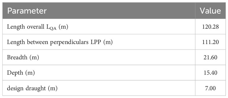
Table 1 Main dimensions of the main hull.

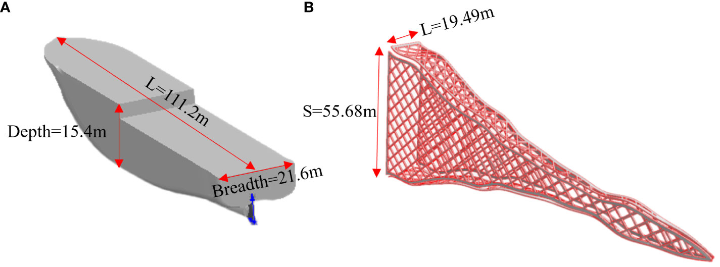
Figure 2 Geometric model of the Antarctic krill ship (A) and the middle trawl (B).

In accordance with the pertinent literature (Lu, 2018), the dimensions of the rectangular cuboid computational domain were as follows: [−2.5LPP, 2.5LPP] in the longitudinal and transverse directions, and [−2LPP, LPP] in the vertical direction. The width and length of the ice-crushing channel were 2LPP and 10LPP, respectively.

The boundary settings for the computational domain were set as follows. A velocity inlet was located at 1.5 times the captain’s position in front of the bow, with the velocity at the inlet being equal to the VOF wave velocity. A pressure outlet was located at 2.5 times the captain’s position behind the stern of the ship; the fluid static pressure was the pressure field function, which indicated a fully developed fluid flow. A symmetric plane was located on the left and right sides of the computational domain. A velocity inlet was located at the top of the computational domain. To simulate an infinite water depth, another velocity inlet was located at the bottom of the computational domain. The non-slip wall boundary condition was applied to the surface of the ship.

According to the relevant literature, the grid size of the hull was set to 0.058m. Grid refinement was applied at the boundary of the computational domain and at the bow, stern, and waterline, where the hull collided with sea ice. Figure 3 shows the model grid distribution.

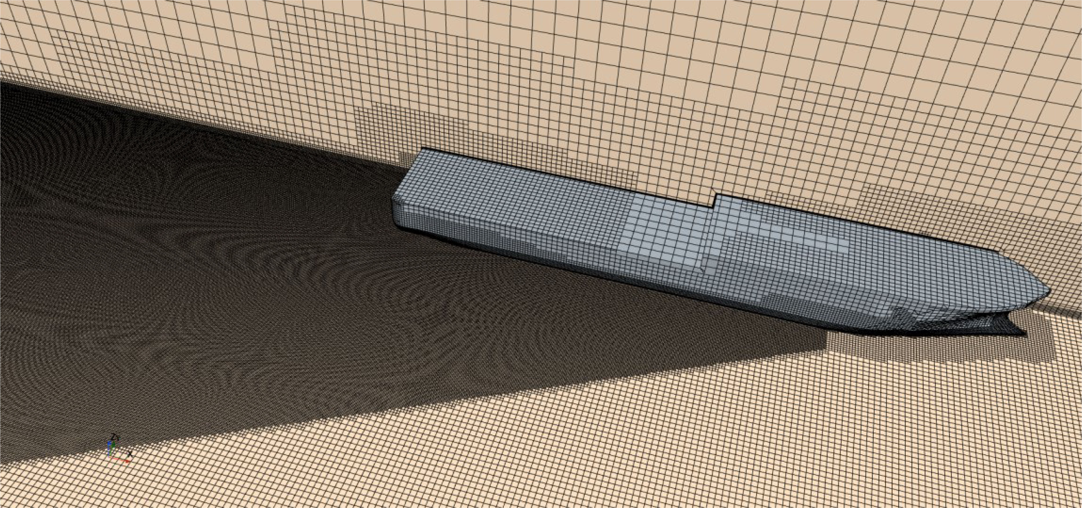
Figure 3 Finite element model of the krill ship and surrounding waters.

About Numerical analysis of the trawl net (Figure 4A), because of the fluid structure interaction in the simulation, a fluid structure interface was created through the contact between the fluid and the mesh. To address the problem of fluid structure interaction, data were exchanged between the fluid region and the solid region at a shared interface, and the displacement and resistance of the mesh were evaluated (see Figure 4B).

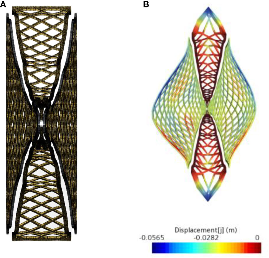
Figure 4 Finite element model of the middle trawl, (A) mesh of the middle trawl; (B) displacement of the middle trawl.

Given the Lagrangian definition of ice particles, physical models that included cylindrical particles, DEM particles, solid particles, and constant-concentration particles were required in the simulation. The selected material of ice was floating ice in Antarctica, and the corresponding ice condition was biennial ice (Daley, 2000; IACS, 2016), with the ice thickness being 0.6 m. Table 2 lists the numerical simulation parameters of a discrete-element model of floating ice.

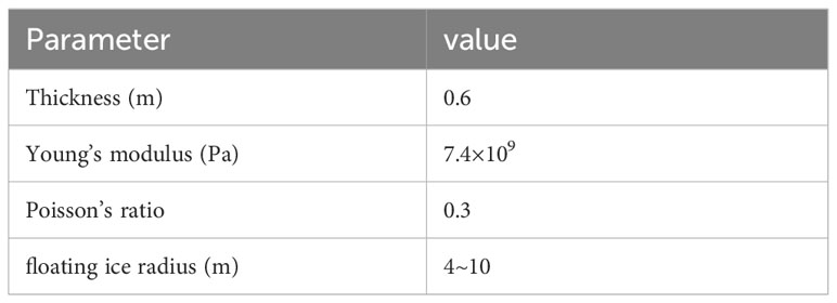
Table 2 Main parameters of a discrete-element model of floating ice.

In this simulation, the pack ice unit was assumed to be unbreakable. A numerical model of floating and broken ice was established by DEM with the hull and floating-ice wall considered to be rigid (Wang et al., 2022). Figure 5 shows an Antarctic krill ship navigating through a polar ice channel. In accordance with relevant statistics (Tuovinen, 1979), the area of the ice flows considerably differed, and the ice flow distribution was excessively random. The area of the ice flows obeyed a lognormal distribution function.

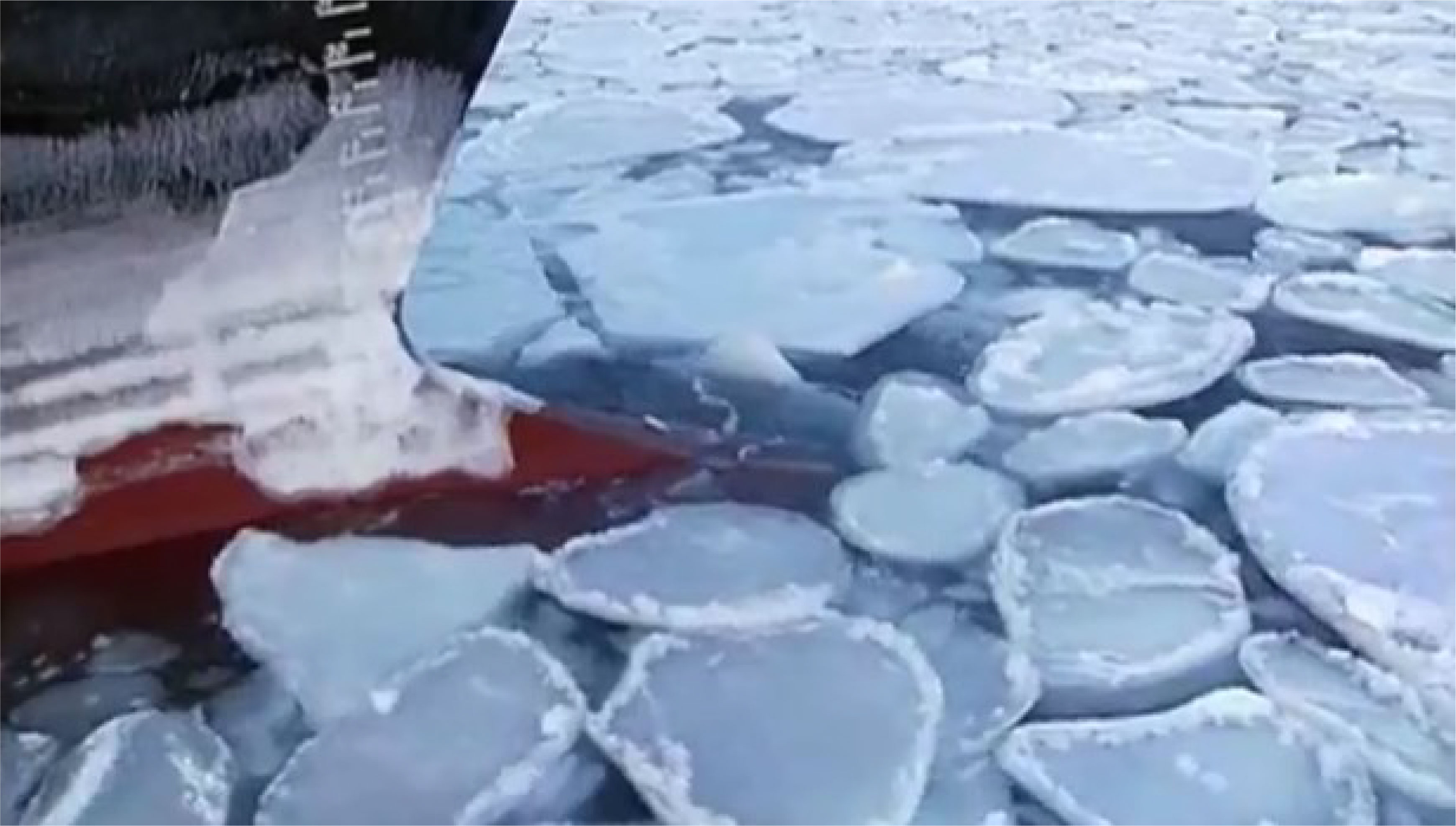
Figure 5 Antarctic krill ship navigating through a polar ice channel.

To achieve a completely random arrangement of ice particles, we used the genetic algorithm in MATLAB to generate the center and radius of an ice circle, and the data were then imported into STAR-CCM+. In brief, the boundary region and radius of a random circle were defined. If the boundary area did not overlap with other circles, it was retained. By contrast, if the boundary area overlapped with other circles, it was excluded, and new center points were created. These operations were repeated until the required ice flow concentration was achieved. Figure 6 shows the arrangement of floating ice, and Figure 7 depicts the distribution of the floating-ice area, which is essentially identical to a lognormal distribution. To facilitate the movement of the entire arrangement of floating ice towards the ship, the velocity of each ice particle was adjusted to match that of the water flow.

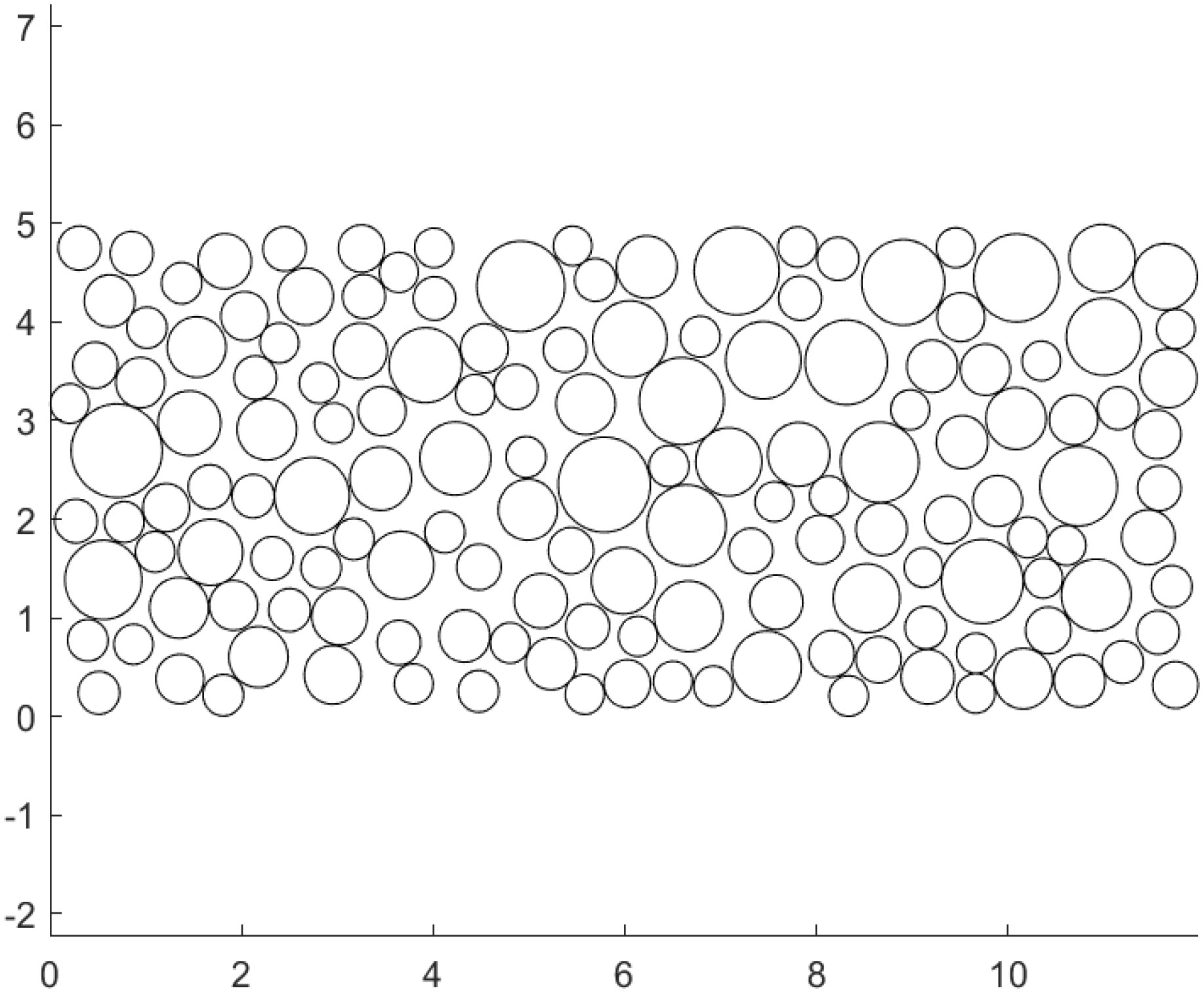
Figure 6 Array of floating ice at a concentration of 60%.

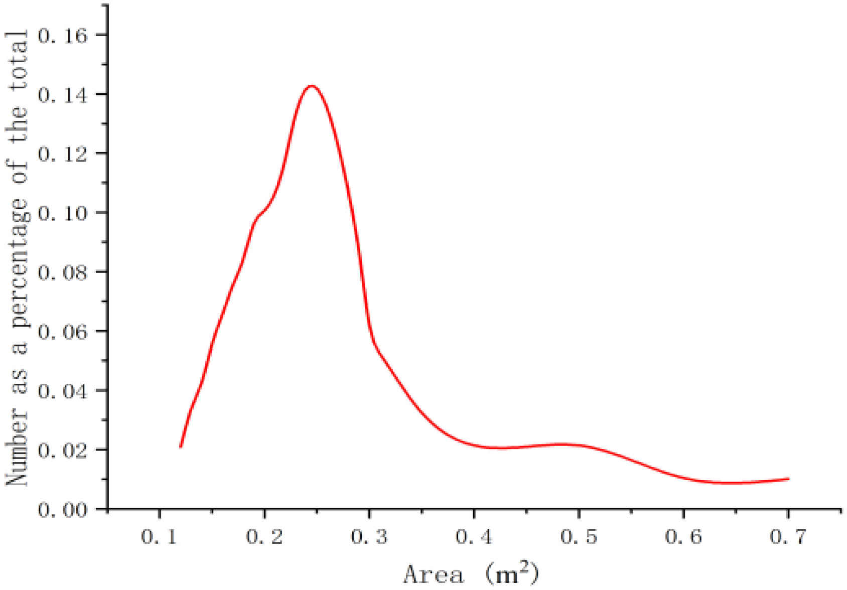
Figure 7 Distribution of the floating-ice area in the simulation.

If the entire floating-ice field flowed past the initial position where it was created, a new floating-ice field was created at the same position. As shown in Figure 8, the ship repeatedly sailed in the ice flow area within a limited computational domain, thus considerably reducing the computational cost.

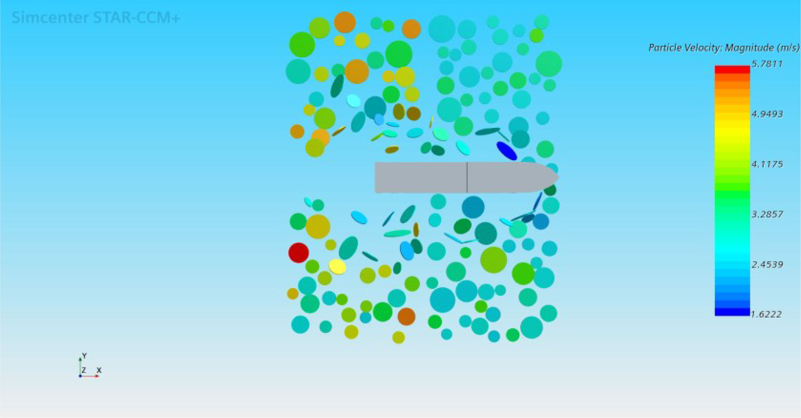
Figure 8 Continuous generation of floating ice array.

3 Results

3.1 Validation and verification

First, the time step and grid convergence analysis was performed. Three different time steps and grids were selected for analysis, and the unified refinement ratio of the grid was √2, which was recommended by the ITTC committee. As shown in Equations 20 and 21, the corresponding numerical solutions of the triple grid were fine solution SG 1, medium solution SG 2 and coarse solution SG 3, respectively, and the difference of numerical solutions of the two sets of adjacent grids was calculated.approach:

The convergence factor RG is calculated according to equation (10) to determine the convergence of the numerical solution: if 0<RG<1, the numerical solution converges monotonically; if RG<0, the numerical solution converges; if RG> 1, the numerical solution diverges.

The specific values of the time steps and grids and their corresponding water resistance are shown in Tables 3 and 4. Considering the accuracy of the simulation results and the efficiency of the calculation, the time step 2 grid case 2 were selected for calculation.

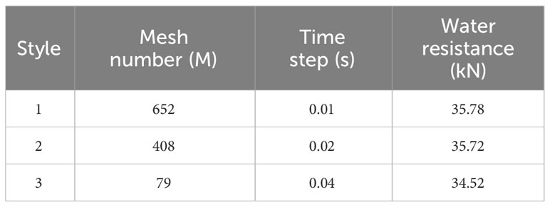
Table 3 Convergence analysis for the ship hull.

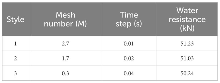
Table 4 Convergence analysis for the middle trawl Style.

Figure 9 presents a comparison of the simulated water resistance obtained in the present study with the pool test data obtained from experimental trawl model tests conducted by Zhipeng in the hydrodynamic circulating tank of Tokyo University. Figure 10 illustrates the resistance test for the krill ship model. Their scale-reduction ratios were 1:35 and 1:25, respectively. Further details on these tests can be found in (Su, 2017). As illustrated in Figures 11 and 12, the experimental values were generally larger than the simulation values, presumably due to the constant velocity assumed in the simulation. However, in an actual experimental environment, maintaining a constant velocity is unfeasible, particularly in a drift-ice region. Therefore, to maintain a constant velocity, the tractive force of the model ship should be considerably larger than that assumed in the simulation. In the present study, the maximum errors in water resistance for the main hull and trawl were approximately 11.7%. Therefore, the simulation results are in close agreement with the test results, which indicates that the developed model ship was reliable in predicting resistance and simulating the driving process in ice areas.

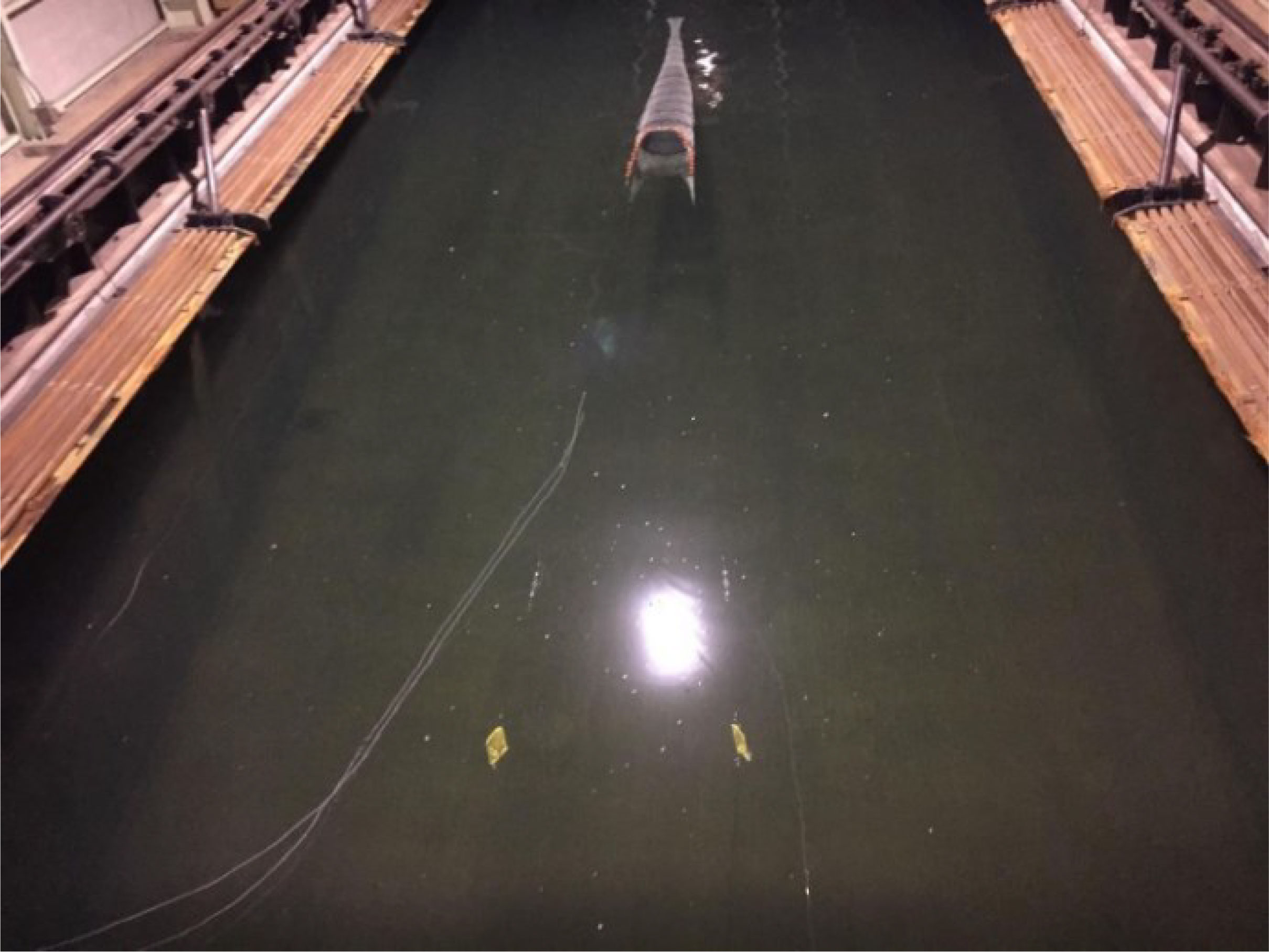
Figure 9 Trawl model test.

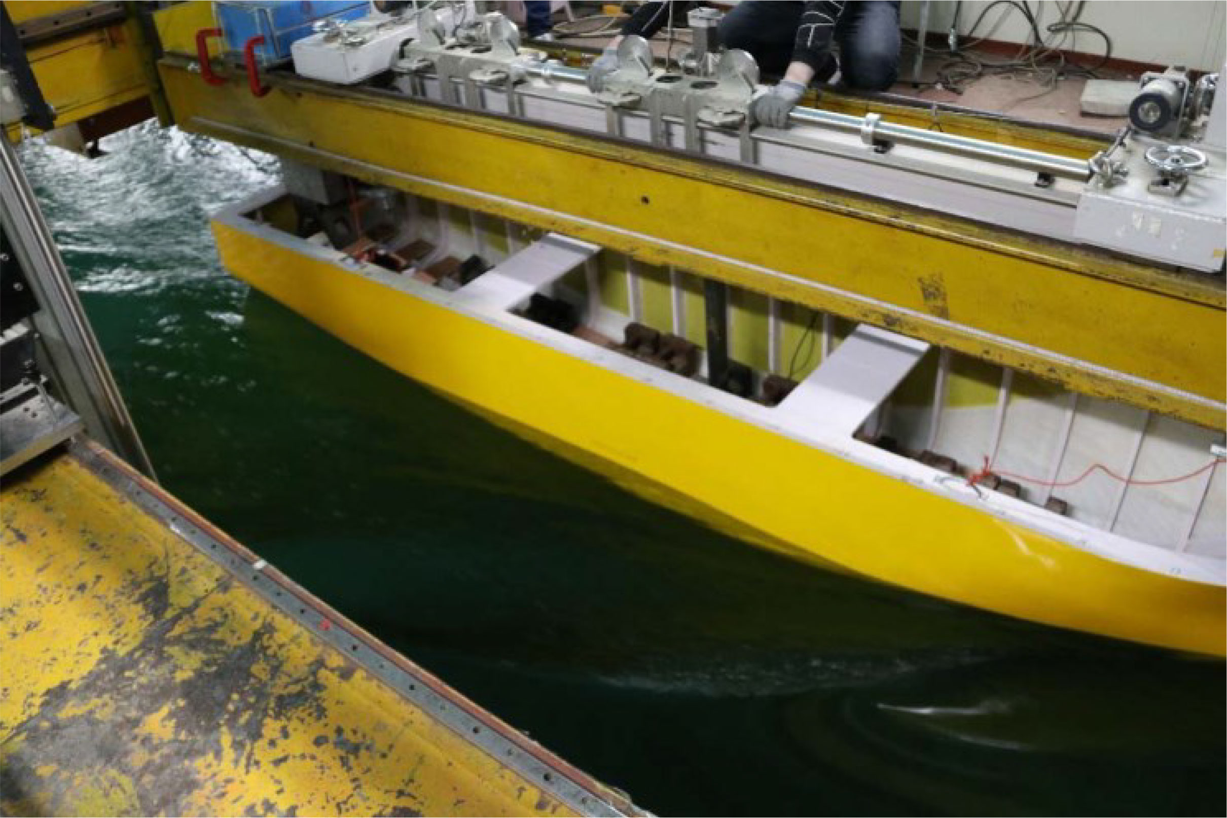
Figure 10 Krill ship model test.

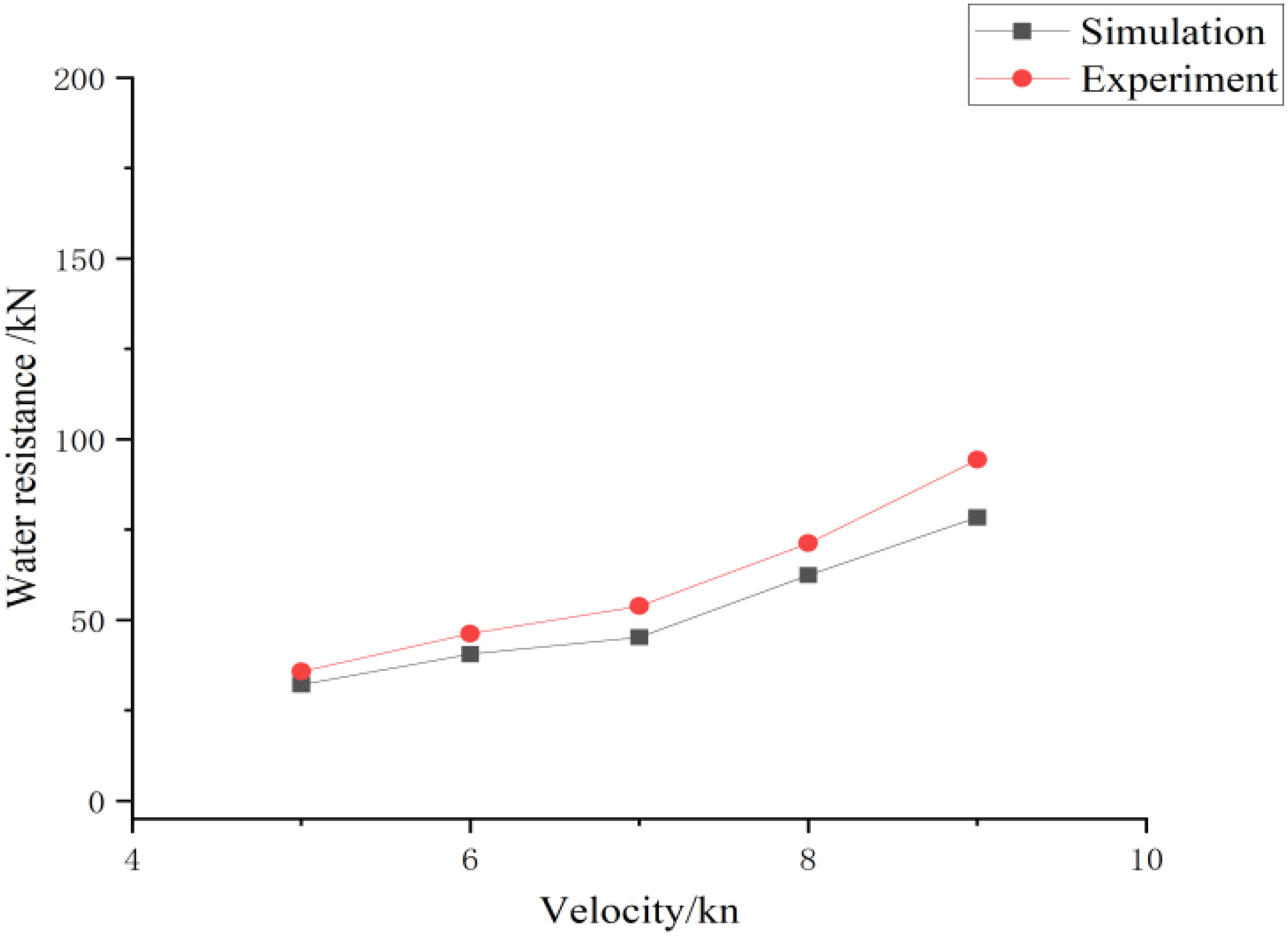
Figure 11 Comparison of resistance for the Antarctic krill ship.

Figure 12 Comparison of resistance for the middle trawl.

3.2 Numerical calculation results and analysis

3.2.1 Analysis and comparison of ice resistance

Given the influence of floating ice speed and concentration on ice resistance, simulations were conducted at five speeds: 5, 6, 7, 8, and 9kn. These simulations were conducted at ice flow concentrations of 40%, 50%, and 60%. Figure 13 depict the ice resistance under various operating conditions, which represents the force that hinders the navigation of ships caused by the collision between ice and the hull.

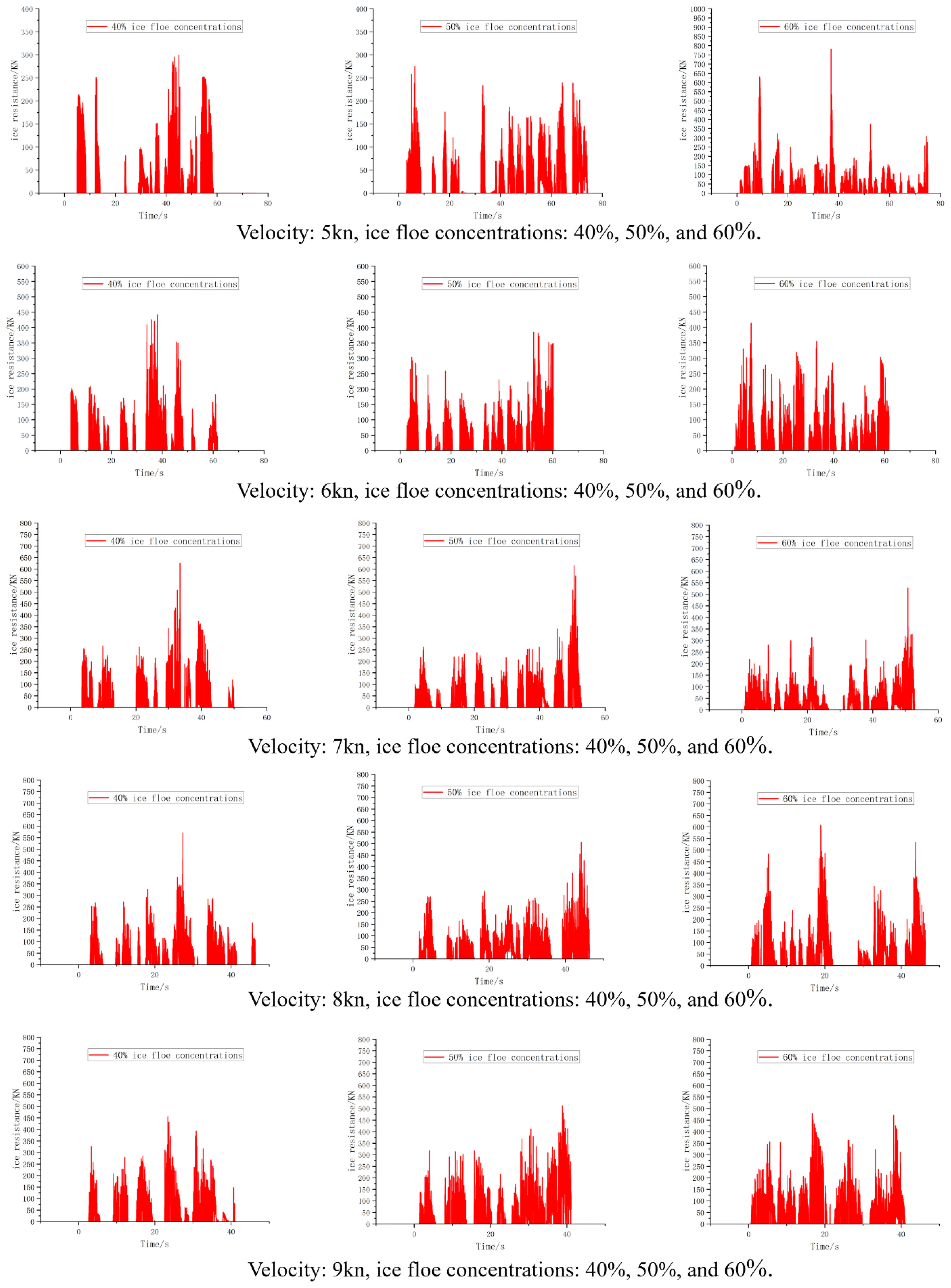
Figure 13 Ice resistance at five ship speeds and three ice flow densities.

Figure 14 depicts ship navigation scenarios with varying ice flow concentrations. As illustrated in Figure 14, part A, at a sailing speed of 5kN and an ice flow concentration of 40%, some of the drift ice collided with the bow of the ship and slid for a certain distance as it flowed towards the ship. The fast current observed in the wake region affected this drift ice and caused it to flow, spin, and increase its speed while simultaneously colliding with other pieces of drift ice. However, not all drift ice collided with the bow of the ship; some of the floating ice collided with other areas of the ship, thereby generating friction. As a consequence of the compression and collision experienced by the ship, the drift ice on the bow of the model ship concentrated against the hull, thereby leading to the formation of a changing area (with concentrated drift ice) as wide as the model ship on both sides of the vessel.

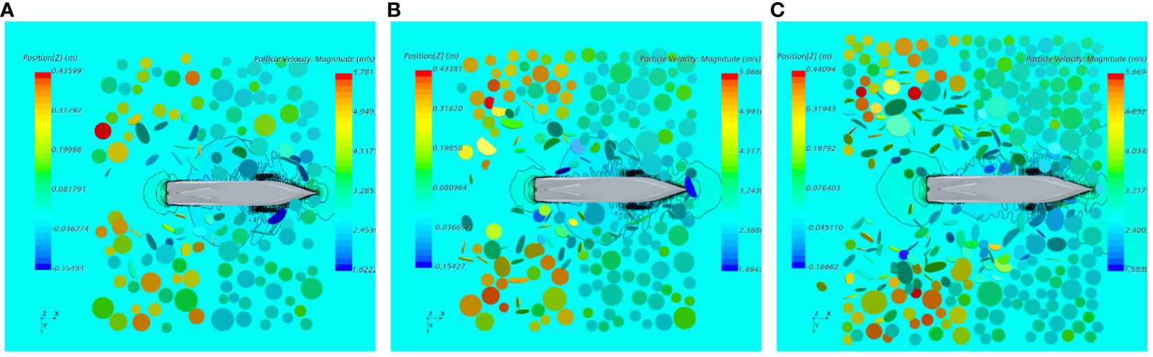
Figure 14 Ship navigation scenario, (A) ice flow concentration of 40%; (B) ice flow concentration of 50%; (C) ice flow concentration of 60%.

Overall, the discontinuity observed in the force exerted by floating ice on the ship was attributable to the collisions between the floating ice and the ship, which led to overturning. Consequently, collisions with other pieces of floating ice occurred, which disrupted the original arrangement of floating ice and created a gap within the arrangement. For ships navigating through sea ice, ice resistance plays an essential role in determining their service life. In this study, ice resistance diagrams for different speeds and densities of drift ice were used to calculate the average ice resistance. Figure 15 depicts the variation in the ice resistance with the ice flow concentration at different speeds.

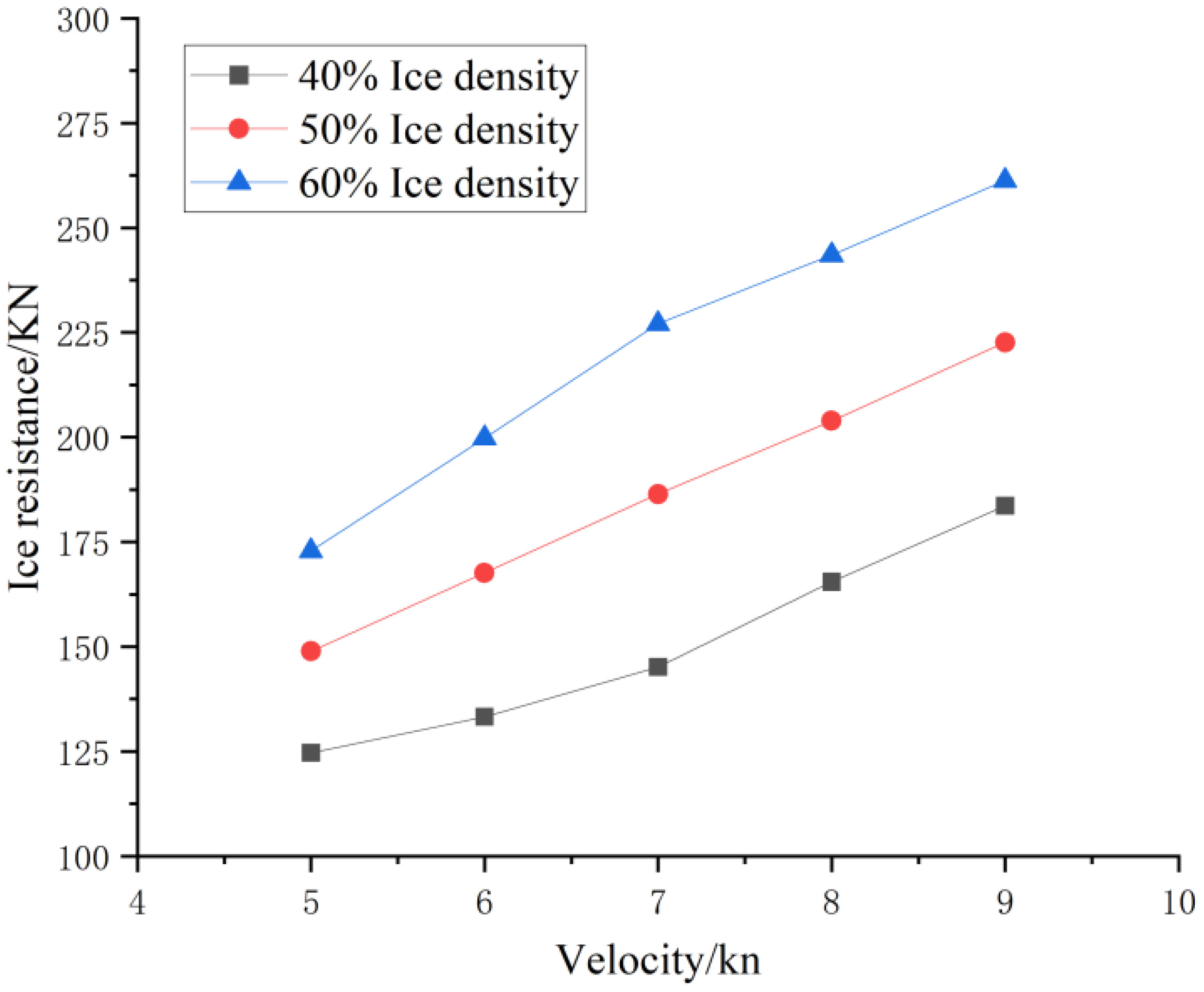
Figure 15 Ice resistance versus speed at various ice flow concentrations.

As shown in Figure 15, ice resistance positively correlated with ice flow concentration and velocity. Under various conditions, the increase observed in ice resistance followed a regular pattern. The ice resistance at an ice flow concentration of 40% was used as a standard rate to calculate the variation in ice resistance with the ice density (see Table 5).

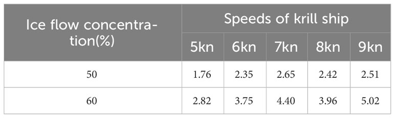
Table 5 Difference in ice resistance at various ice flow concentrations.

As presented in Table 5, the difference in ice resistance at low speeds was small, whereas the difference in ice resistance at high speeds was relatively large. At low speeds, the ice flows were slowly pushed by the ship to either side. However, at high speeds, the ice flows were rapidly pushed away from the ship, which was accompanied by the overturning and sinking of the ice flows.

At a speed of 7kn, the friction between the hull and the ice flows and the water resistance of the ice flows balanced each other, which resulted in a blockage at points where the ship was unable to push the ice flows away. Thus, the difference in ice resistance increased.

As demonstrated in Table 6, the ratio of ice resistance to water resistance exhibited an inverse relationship with drift ice concentration at a constant speed. Conversely, at a constant concentration of drift ice, the ratio of ice resistance to water resistance exhibited a direct relationship with speed. This phenomenon can be attributed to the fact that the water resistance surpassed the drift ice resistance with increasing speed, which led to a decrease in the ratio of ice resistance to water resistance.

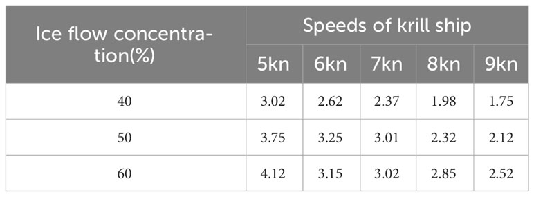
Table 6 Ratio of ice resistance to water resistance at various ice flow concentrations.

3.2.2 Analysis of total resistance

The total resistance experienced by the Antarctic krill ship while navigating through the ice flow area was determined by combining the drag net resistance, water resistance, and ice resistance endured by the main hull. Figure 16 depicts the total resistance encountered by the Antarctic krill ship at different ice flow concentrations.

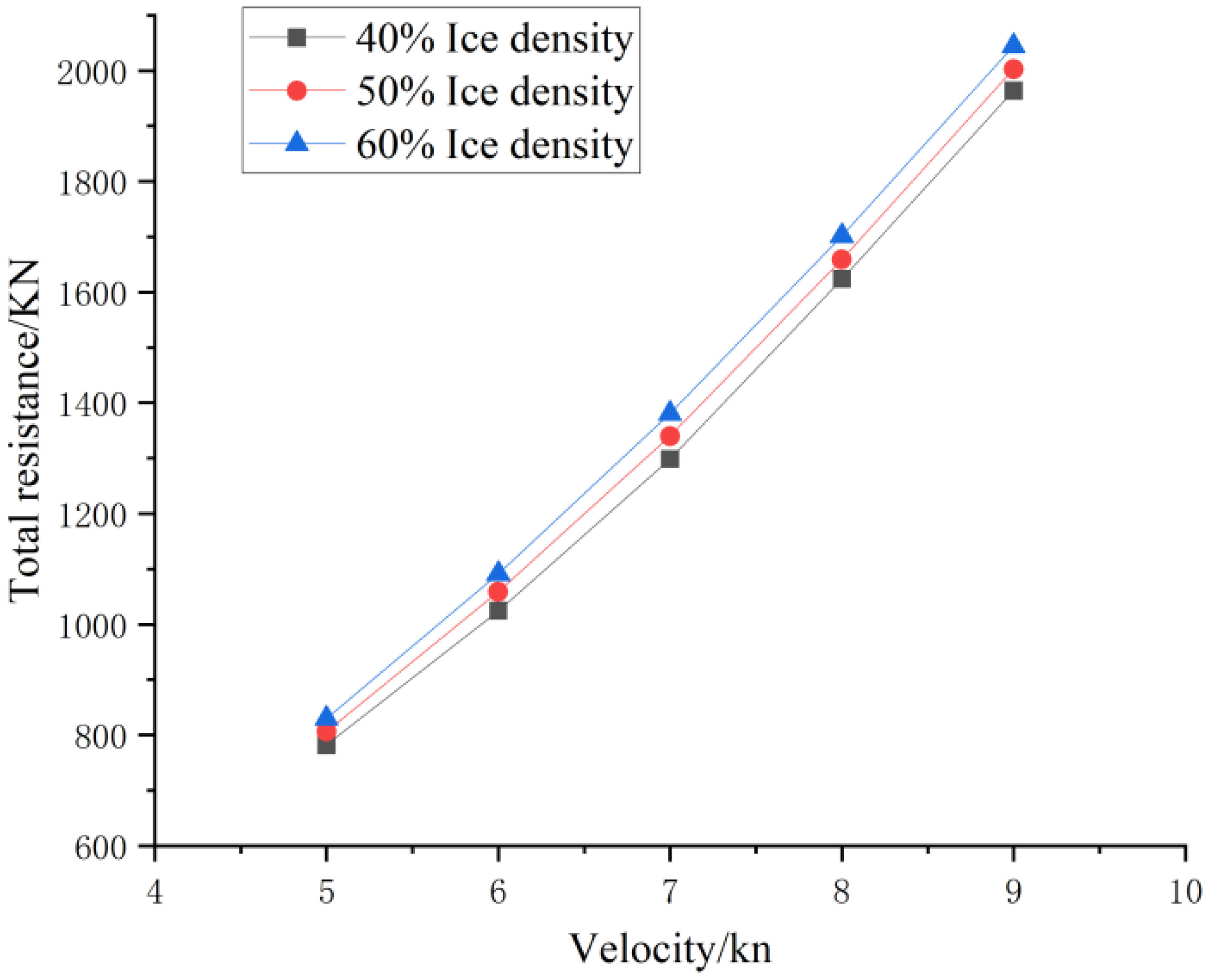
Figure 16 Total resistance encountered by the Antarctic krill ship at different ice flow concentrations.

The growth rate of total resistance at different ice flow concentrations was essentially uniform. To analyse the percentage of each force in total resistance, total resistance at an ice flow concentration of 50% was selected.

As presented in Table 7, when speed increased, the percentages of water resistance and trawl resistance in the total resistance increased by approximately 5% and 8%, respectively, and the percentage of ice resistance in the total sample decreased by approximately 10%. Moreover, the increase in water resistance is faster than that of trawl resistance. In summary, trawl resistance is the main component of total resistance. Therefore, adopting an appropriate trawl design can effectively reduce the total resistance of Antarctic krill vessels while sailing through ice flows.

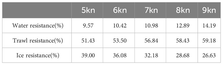
Table 7 Percentage of each force in the total resistance at an ice flow concentration of 50%.

4 Discussion

Antarctic krill resources in the Southern Ocean present significant opportunities for the fisheries industry. State-of-the-art specialized fishing and processing vessels play a crucial and necessary role in Antarctic krill harvesting. As the China Classification Society (CCS) and the fishery department have very strict requirements on the construction and operation of Antarctic krill ships, to ensure that these ships can safely and effectively catch krill in the extremely harsh Antarctic environment. Ships shall meet the special requirements of polar waters, including low temperature, ice collision, wind and waves, etc. The ship structure shall be strong enough to withstand the effects of extreme weather and ice conditions to ensure the safety of the hull and equipment. The ship shall have sufficient stability and wave resistance to ensure operational safety and crew comfort in harsh sea conditions. Therefore, this study uses numerical simulation method to study the resistance encountered by vessels and trawls in ice-invaded waters, and solves the practical challenge of floating ice floating in the working area of Antarctic krill vessels. The effectiveness of numerical simulations based on the CFD-DEM method is evaluated by comparing with the experimental results of laboratory models.

Presently, research on Antarctic krill trawl nets primarily focuses on the mesh design and the simulated catch volume’s impact on net performance. Few studies, however, have examined the ice resistance capabilities of Antarctic krill vessels and the overall resistance of the unified system consists of the vessel and trawl net during navigation. This is the main task of this paper to address and discuss. The study reveals that higher speeds do not necessarily guarantee smoother vessel navigation. At a speed of 7kn, the friction and water resistance between the ship and the ice flows can sometimes reach an equilibrium, leading to the buildup of ice flows. With speed increasing, the total resistance experienced by the vessel rises, with a decrease in the proportion of ice resistance and an increase in trawl net resistance.

The Southern Ocean exhibits complex sea conditions, with perennial ice and a diverse array of ice types, each with intricate properties. Ice flows encountered in navigable channels extend beyond simple pancake-shaped ice. The numerical simulation in this paper utilizes cylinders of varying diameters to approximately simulate ice flows, simplifying the real scenario for computational efficiency. A more detailed analysis and assumptions about the shape and other physical properties of ice flows would provide meaningful insights, allowing simulations to better align with real conditions and identify key factors influencing vessel navigation.

The results of numerical simulation methods rely on computer hardware, model selection and parameter settings. Despite its dependency on these factors, numerical simulation technology, which has been enhanced by improvements in artificial intelligence and big data, presents significant advantages in terms of time-efficiency and cost savings compared to model and sea trials. It is anticipated that numerical simulation techniques will be adapted to broader applications and yield more accurate results in the design, manufacture and operation of ships and other structures, facilitated by developments in computer technology. This paper offers insights and reflections on the research of ice resistance in vessels and serves as a reference for the travelling speed of Antarctic krill fishing vessels engaged in fishing.

5 Conclusion

In this study, the navigation process of Antarctic krill vessels through polar ice flows was simulated, and the effects of ice flows on various parts of these vessels and their movement after the collision were analyzed. In addition, the navigation process of Antarctic krill vessels at different velocities and concentrations of ice flows was examined. The main conclusions of this study are as follows:

(1) The pattern of collision between floating ice and a vessel differs depending on the vehicle’s speed. At a low speed, floating ice is slowly pushed aside by the ship, whereas at a high speed, floating ice is rapidly crushed by the ship, thereby causing the ice to overturn and sink.

(2) At a speed of 7kn the friction between the hull and ice flows and the water resistance sometimes reaches equilibrium. Therefore, floating ice will accumulate around the bow of ship, resulting in the increase of ice resistance.

(3) Trawl resistance is the main component of the total resistance experienced by Antarctic krill vessels. As opposed to ice resistance, the proportion of trawl resistance to total resistance continues to increase as the ship speed increases.

Data availability statement

The original contributions presented in the study are included in the article/supplementary material. Further inquiries can be directed to the corresponding author.

Author contributions

ZX: Conceptualization, Writing – original draft, Writing – review & editing. XW: Data curation, Writing – original draft. YG: Software, Validation, Writing – review & editing. ZF: Supervision, Writing – review & editing.

Funding

The author(s) declare that no financial support was received for the research, authorship, and/or publication of this article.

Acknowledgments

The authors are grateful to the Shanghai Engineering Technology Research Centre of Deep Offshore Material (19DZ2253100).

Conflict of interest

The authors declare that the research was conducted in the absence of any commercial or financial relationships that could be construed as a potential conflict of interest.

Publisher’s note

All claims expressed in this article are solely those of the authors and do not necessarily represent those of their affiliated organizations, or those of the publisher, the editors and the reviewers. Any product that may be evaluated in this article, or claim that may be made by its manufacturer, is not guaranteed or endorsed by the publisher.

References

Cai J., Ding S., Zhang Q., Liu R., Zeng D., Zhou L. (2022). Broken ice circumferential crack estimation via image techniques. Ocean Eng. 259, 111735. doi: 10.1016/j.oceaneng.2022.111735
Chen J., Kang S., Du W., Guo J., Xu M., Zhang Y., et al. (2021). Perspectives on future sea ice and navigability in the Arctic. Cryosphere. 15, 5473–5482. doi: 10.5194/tc-15-5473-2021
Cheng J., Song W., Li, Li L., Yang J., Rao X., et al. (2022). The influence of the structural change of the mesh opening on the hydrodynamic performance of the antarctic krill truss trawl. Fish. Modern. 49 (4), 96–103. doi: 10.3969/j.issn.1007-9580.2022.04.012
Coetzee C. J. (2016). Calibration of the discrete element method and the effect of particle shape. Powder Technol. 297, 50–70. doi: 10.1016/j.powtec.2016.04.003
Dai K., Li Y., Gong J., Fu Z., Li A., Zhang D. (2022). Numerical study on propulsive factors in regular head and oblique waves. Brodogradnja. 73, 37–56. doi: 10.21278/brod73103
Daley C. (2000). “IACS Unified requirement for polar ships: background notes to design ice loads,” in Technical Report Prepared for IACS Adhoc Group on Polar Class Ships, Transport Canada, vol. 186. , 106114.
Das J. (2017). Modeling and validation of simulation results of an ice beam in four-point bending using smoothed particle hydrodynamics. Int. J. Offshore Polar Eng. 27, 82–89. doi: 10.17736/10535381
Erceg S., Ehlers S. (2017). Semi-empirical level ice resistance prediction methods. Ship Technol. Res. 64, 1–14. doi: 10.1080/09377255.2016.1277839
Georgiev P., Garbatov Y. (2021). Multipurpose vessel fleet for short black sea shipping through multimodal transport corridors. Brodogradnja 72, 79–101. doi: 10.21278/brod72405
Guan Q., Zhu W., Zhou A., Wang Y., Tang W., Wan R. (2022). Numerical and experimental investigations on hydrodynamic performance of a newly designed deep bottom trawl. Front. Mar. Sci. 9. doi: 10.3389/fmars.2022.891046
Guo C. Y., Xie C., Zhang J. Z., Wang S., Zhao D. G. (2018a). Experimental investigation of the resistance performance and heave and pitch motions of ice-going container ship under pack ice conditions. China Ocean Eng. 32, 169–178. doi: 10.1007/s13344-018-0018-9
Guo C. Y., Zhang Z. T., Tian T. P., Li X., Zhao D. (2018b). Numerical simulation on the resistance performance of ice-going container ship under brash ice conditions. China Ocean Eng. 32, 546–556. doi: 10.1007/s13344-018-0057-2
Gutfraind R., Savage S. B. (1998). Flow of fractured ice through wedge-shaped channels: smoothed particle hydrodynamics and discrete-element simulations. Mech. Mater. 29, 1–17. doi: 10.1016/S0167-6636(97)00072-0
Han Y. (2021). Research on damage stability of arctic navigation ships (Liaoning Province, China: Dalian University of Technology), 001115.
Huang L., Li F., Li M., Khojasteh D., Luo Z., Kujala P. (2022). “An investigation on the speed dependence of ice resistance using an advanced CFD+DEM approach based on pre-sawn ice tests,”, vol. 264. (Elsevier Press: Ocean Eng), 112530. doi: 10.1016/j.oceaneng.2022.112530
Huang Y., Sun J. Q., Ji S. P., Tian Y. K. (2016). Experimental study on the resistance of a transport ship navigating in level ice. J. J. Mar. Sci. Appl. 15, 105–111. doi: 10.1007/s11804-016-1351-0
IACS (2016). Requirements concerning polar class Vol. 6 (Oslo, Norway: International Association of Classification Societies), 211–221.
Jiménez-Herrera N., Barrios G. K. P., Tavares L. (2018). Comparison of breakage models in dem in simulating impact on particle beds. Adv. Powder Technol. 29, 692–706. doi: 10.1016/j.apt.2017.12.006
Kim J. H., Kim Y., Kim H. S., Jeong S. Y. (2019). Numerical simulation of ice impacts on ship hulls in broken ice fields. Ocean Eng. 180, 162–174. doi: 10.1016/j.oceaneng.2019.03.043
Kim M. C., Lee S. K., Lee W. J., Wang J. Y. (2013). Numerical and experimental investigation of the resistance performance of an icebreaking cargo vessel in pack ice conditions. Int. J. Nav. Archit. Ocean Eng. 5, 116–131. doi: 10.2478/IJNAOE-2013-0121
Kim M. C., Lee W. J., Shin Y. J. (2014). Comparative study on the resistance performance of an icebreaking cargo vessel according to the variation of waterline angles in pack ice conditions. Int. J. Nav. Archit. Ocean Eng. 6, 876–893. doi: 10.2478/IJNAOE-2013-0219
Koto J., Afrizal E. (2017). Empirical approach to predict ship resistance in level ice. J. Ocean Eng. Mar. Energy. 45, 1–8.
Lau M., Lawrence K. P., Rothenburg L. (2011). Discrete element analysis of ice loads on ships and structures. Ships Offshore Struct. 6, 211–221. doi: 10.1080/17445302.2010.544086
Lewis J. W., Debord F. W., Bula V. A. (1982). Resistance and propulsion of ice worthy ships. Trans. – Soc Nav. Archit. Mar. Eng. 90, 249–276.
Lu X. (2018). Ice load calculation of Icebreaker based on near-field dynamics and finite element coupling (Harbin, Heilongjiang Province, China: Harbin Engineering University), 000224.
Norouzi H., Zarghami R., Sotudeh-Gharebagh R., Mostoufi N. (2016). Couple CFD-DEM modeling: formulation, implementation and application to multiphase flows Vol. 165 (Hoboken, New Jersey: Wiley Online Library), 752–770.
Patricio A., Renzo R., Álvaro D. C. (2016). Chilean Antarctic krill fishery. Lat. Am. J. Aquat. Res. 48, 179–196.
Polojärvi A., Tuhkuri J. (2013). On modeling cohesive ridge keel punch through tests with a combined finite-discrete element method. Cold Reg. Sci. Technol. 85, 191–205. doi: 10.1016/j.coldregions.2012.09.013
Rod C., Graeme M., Andrew C. (2022). Research funding and economic aspects of the Antarctic krill fishery. Mar. Policy. 143, 105200. doi: 10.1016/j.marpol.2022.105200
Shen H. T., Su J., Liu L. (2000). SPH simulation of river ice dynamics. J. Comput. 165, 752–770. doi: 10.1006/jcph.2000.6639
Su Z. (2017). Analysis on Antarctic krill Mid-water trawl performance based on field measurement and model experiment Vol. 32 (Shanghai, China: Shanghai Ocean University), 169–178.
Sun Q., Zhang M., Zhou L., Garme K., Burman M. (2022). A machine learning-based method for prediction of ship performance in ice: Part I. ice resistance. Mar. Struct. 83, 103181. doi: 10.1016/j.marstruc.2022.103181
Tan X., Su B., Riska K., Moan T. (2013). A six-degrees-of-freedom numerical model for level ice–ship interaction. Cold Reg. Sci. Technol. 92, 1–16. doi: 10.1016/j.coldregions.2013.03.006
Tang H., Nsangue B. T. N., Pandong A. N., He P., Liu X., Hu F. (2022). Flume tank evaluation on the effect of liners on the physical performance of the antarctic krill trawl. Front. Mar. Sci. 8. doi: 10.3389/fmars.2021.829615
Thomson J., Ackley S., Girard-Ardhuin F., Ardhuin F., Babanin A., Boutin G., et al. (2018). Overview of the Arctic Sea state and boundary layer physics program. J. Geophys. 123, 8674–8687. doi: 10.1002/2018JC013766
Tuovinen P. (1979). The size distribution of ice blocks in a broken channel. Teknillinen korkeakoulu. 180, 162–174.
Walton K. (1987). The effective elastic moduli of a random packing of spheres. J. Mech. Phys. Solids. 35, 213–226. doi: 10.1016/0022-5096(87)90036-6
Wang B., Liu Y., Zhang J., Shi W., Li X., Li Y. (2022). Dynamic analysis of offshore wind turbines subjected to the combined wind and ice loads based on the cohesive element method. Front. Mar. Sci. 9. doi: 10.3389/fmars.2022.956032
Wang Z., Tang H., Herrmann B., Xu L. (2021). Catch pattern for antarctic krill (Euphausia superba) of different commercial trawls in similar times and overlapping fishing grounds. Front. Mar. Sci. 8. doi: 10.3389/fmars.2021.670663
Xie C., Zhou L., Ding S., Liu R., Zheng S. (2023). Experimental and numerical investigation on self-propulsion performance of polar merchant ship in brash ice channel. Ocean Eng. 269, 113424. doi: 10.1016/j.oceaneng.2022.113424
Yang G., Atkinson A., Hill S. L., Guglielmo L., Granata A., Li C. (2020). Changing circumpolar distributions and isoscapes of Antarctic krill: Indo-Pacific habitat refuges counter long-term degradation of the Atlantic sector. Limnol. Oceanogr. 66 (1), 1–16. doi: 10.1002/lno.11603
Zhao G. (2016). Ice load calculation of Icebreaker based on near-field dynamics (Harbin, Heilongjiang Province, China: Harbin Engineering University), 108–119.
Zhong W., Yu C. Y., Wen Y. T. (2023). Experimental investigation on ice resistance of an arctic LNG carrier under multiple ice breaking conditions. Ocean Eng. 267, 113264. doi: 10.1016/j.oceaneng.2022.113264
Zhu M., Tang H., Liu W., Zhang F., Sun Q., Xu L., et al. (2023). Effects of different horizontal expansion ratios and simulated catches on the overall shape of Antarctic krill trawl. J. Dalian Ocean University. 38 (2), 331–339. doi: 10.16535/j.cnki.dlhyxb.2022-188
Keywords: Antarctic krill ship, resistance characteristic, floating ice, trawl, numerical simulation
Citation: Xiong Z, Wu X, Guo Y and Fu Z (2024) Study on ice resistance of Antarctic krill ship with trawl under floating ice sea conditions. Front. Mar. Sci. 11:1357331. doi: 10.3389/fmars.2024.1357331
Received: 26 December 2023; Accepted: 22 April 2024;
Published: 13 May 2024.
Edited by:
Stephen J. Newman, Western Australian Fisheries and Marine Research Laboratories, AustraliaReviewed by:
Changqing Jiang, University of Duisburg-Essen, GermanyYen-Chiang Chang, Dalian Maritime University, China
Copyright © 2024 Xiong, Wu, Guo and Fu. This is an open-access article distributed under the terms of the Creative Commons Attribution License (CC BY). The use, distribution or reproduction in other forums is permitted, provided the original author(s) and the copyright owner(s) are credited and that the original publication in this journal is cited, in accordance with accepted academic practice. No use, distribution or reproduction is permitted which does not comply with these terms.
*Correspondence: Zhixin Xiong, zxxiong@shmtu.edu.cn