Remote sensing estimation of δ¹⁵N_PN in the Zhanjiang Bay using Sentinel-3 OLCI data based on machine learning algorithm

1 Introduction

Nitrogen is one of the main nutrients for marine organisms, and it is the two most basic elements in marine ecosystems along with carbon (Eppley and Peterson, 1979; Falkowski, 1997; Galloway et al., 2004). There is a transformation of nitrogen forms between particulate and dissolved states, and the mutual transformation of different nitrogen forms constitutes a complex marine nitrogen cycle (Pajares and Ramos, 2019). The marine nitrogen cycle is closely related to the carbon cycle, and nitrogen limitation or excess can lead to a decrease or increase in the absorption of CO₂ by phytoplankton, so the nitrogen cycle can indirectly affect climate change by regulating the carbon cycle (Falkowski, 1997; Voss et al., 2013). Consequently, accurately grasping the spatiotemporal characteristics of ocean nitrogen is of great significance for deeply understanding the ocean nitrogen cycle and climate change.

Although particulate nitrogen (PN) only accounts for 0.5% of the total nitrogen pool in the ocean, it has the characteristics of easy degradation and fast cycling speed, and is an important component of the nitrogen pool in the ocean (Capone et al., 2008). The main sources of coastal marine particulate nitrogen include marine phytoplankton production, riverine inputs and sewage effluent, and there are significant differences in the isotopic values of particulate nitrogen from different sources (Montoya et al., 2002; Wu et al., 2007; Lu et al., 2021). Particulate nitrogen isotope (δ¹⁵N_PN) is a potential indicator of particulate organic matter sources, and the contribution ratio of different sources of particulate organic matter can be quantitatively calculated using δ¹⁵N_PN and particulate organic carbon isotope (δ¹³C) (Chen et al., 2021; Huang et al., 2021; Lu et al., 2021). δ¹⁵N_PN can also indicate the pollution of the water environment, as it reflects the source of absorbed nutrients (Sarma et al., 2020). One of the main sources of nitrogen-containing nutrients in coastal waters comes from sewage, and δ¹⁵N_PN is significantly enriched (>10%) for sewage (Sarma et al., 2020). In addition, the variation of particulate nitrogen isotope values is also affected by isotope fractionation during nitrogen conversion processes such as nitrification, denitrification, and biological assimilation absorption (Cifuentes et al., 1988; Granger et al., 2010). Therefore, knowledge of the distribution and variation of δ¹⁵N_PN, and the factors controlling their distribution is essential to elucidate the sources and biogeochemical processes of particulate organic matter (Huang et al., 2020).

The traditional particulate nitrogen isotope values are obtained by collecting in situ water sampling and laboratory determination (Chen et al., 2021; Lu et al., 2021). However, this method is time-consuming, labor-intensive, inefficient, and cannot obtain particulate nitrogen isotope values on a large-scale and for a long-time. It is worth exploring how to more conveniently and effectively obtain particulate nitrogen isotope values. Ocean color remote sensing is a method of retrieving water parameters by establishing a response relationship between the remote sensing reflectance and the water parameters (Wang et al., 2022). It has the advantages of large-scale and long-term continuous observation (Shen et al., 2020). In the past several decades, some environmental parameters in water have been retrieved by remote sensing, such as chlorophyll a (Chl a), total suspended matter (TSM), colored dissolved organic matter (CDOM), total phosphorus (TP), total nitrogen (TN), and dissolved inorganic nitrogen (DIN) (Xu et al., 2010; Ondrusek et al., 2012; Mathew et al., 2017; Du et al., 2018; Watanabe et al., 2018; Shen et al., 2022). Among these retrieving elements, the spectral response of other elements may not be significant compared to Chl a, TSM and CDOM, which makes traditional empirical fitting methods difficult to retrieve (Zheng et al., 2024). Machine learning methods generally produce better performance than simple empirical fitting methods (Liu et al., 2021). Recently, inland, coastal, and oceanic water environments have been studied using machine learning methods (Cao et al., 2020; Liu et al., 2021; Shen et al., 2022; Tian et al., 2024; Maciel et al., 2021; Pahlevan et al., 2020). Machine learning algorithms can not only combine multiple input features that are sensitive to the target variable, but also have stronger fitting ability to capture the relationship between the input variable and the target variable (Liu et al., 2021). Sentinel-3, the third of the Copenhagen mission’s six satellites, is equipped with the most sophisticated water color sensor, the Ocean and Land Color Imager (OLCI) instrument. It will regularly monitor the ocean in almost real-time, with its data being made publicly accessible worldwide. And it has a widespread application in the field of water color remote sensing (Du et al., 2018; Pahlevan et al., 2020; Shen et al., 2020, 2022).

Thus, this study aims to explore the potential of machine learning methods for δ¹⁵N_PN satellite retrieving. To achieve this aim, based on determining the optical indicators for retrieving particulate nitrogen isotope values, and then constructing optimal machine learning retrieval model of δ¹⁵N_PN is applied to the Sentinel-3 OLCI data to obtain spatiotemporal information of δ¹⁵N_PN in the Zhanjiang Bay (a typical eutrophic bay in China). The results from this study could improve the ability of remote sensing monitoring of coastal δ¹⁵N_PN and comprehensively understand the biogeochemical processes of marine nitrogen cycle.

2 Materials and methods

2.1 Study area

Zhanjiang Bay is located in the northwest of the South China Sea and is a typical bay with a small mouth and large belly (Figure 1). The connection between Zhanjiang Bay and the South China Sea is mainly through a narrow channel with a width of approximately 2 km (Zhang et al., 2020b). Zhanjiang Bay is located in the subtropical monsoon climate zone, with a rainy season from April to September, and less rainfall from November to February of the following year (Chen et al., 2019). There are many industrial zones, agricultural zones, aquaculture zones, ports, and densely populated areas along the coast of Zhanjiang Bay. A large amount of industrial and agricultural wastewater and domestic sewage are discharged into the bay, bringing a large amount of nutrients and organic matter to Zhanjiang Bay, which has a certain impact on the ecological environment of Zhanjiang Bay (Zhang et al., 2023). Previous studies have shown that the degree of eutrophication in the water of Zhanjiang Bay is gradually becoming severe (Zhang et al., 2020b).

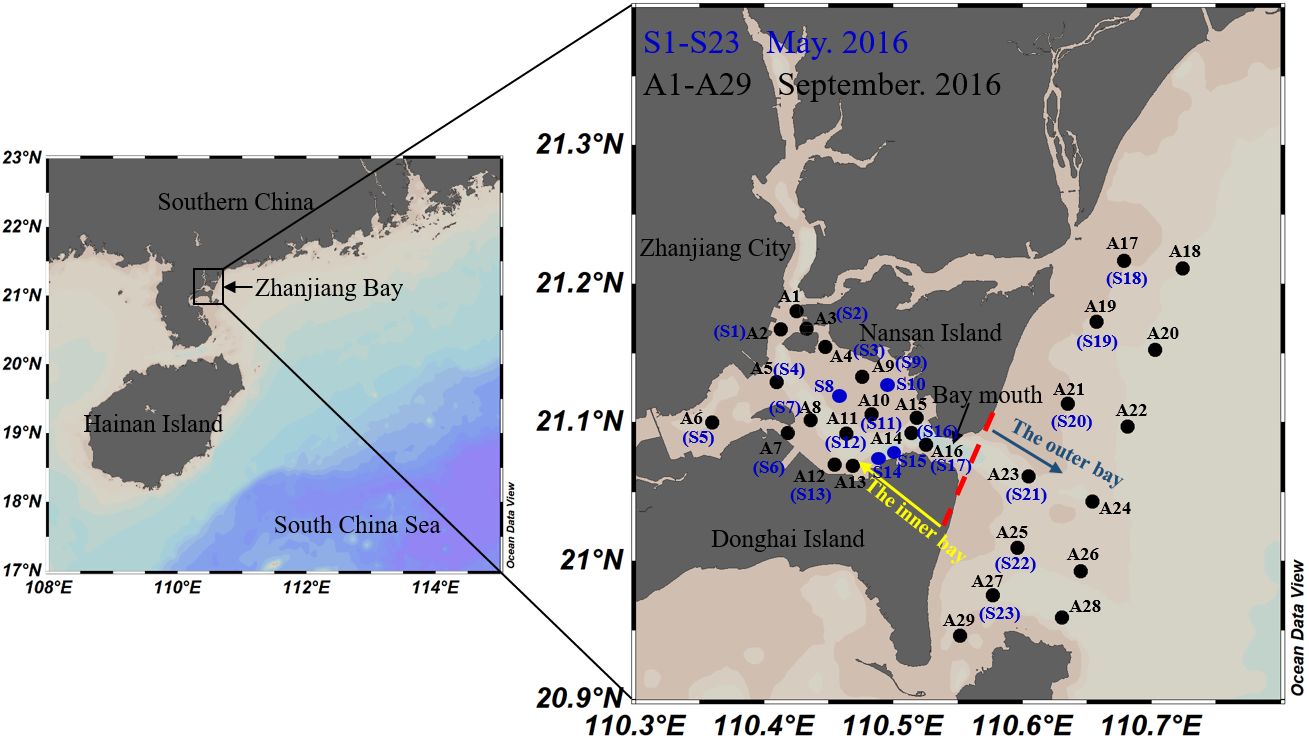
Figure 1 Study area and field sampling stations. S1-S23 and A1-A29 mark the sampling stations in May and September 2016, respectively.

2.2 Field data collection and analysis

The sample collection was conducted in Zhanjiang Bay in May and September of 2016, respectively, with 23 surface water samples collected in May and 29 surface water samples collected in September. The sampling stations are shown in Figure 1. The water samples were placed in polyethylene bottles (each bottle was acid-cleaned and rinsed with ultrapure water) and refrigerated at 4°C in a refrigerator. The water samples were taken back to the laboratory for further analysis on the same day. Furthermore, a spectroradiometer (USB2000+, Ocean Optics, Inc., USA) was used to measure the remote sensing reflectance spectra above the water’s surface between 200 and 1100 nm (1 nm interval) in accordance with the protocols proposed by Mobley (Mobley, 1999). Remote sensing reflectance was determined from an above-water method with an azimuth angle of 135° from the sun and 45° from the nadir (Mobley, 1999). At every water sampling site, the radiances from the sky, the water, and the reference panel were measured. Remote sensing reflectance (R_rs(λ)) was calculated using the following Equation 1:

where λ is the wavelength, L_u(λ) is the upwelling spectral radiance, L_s(λ) is the incident spectral sky radiance and r is the proportionality coefficient, with a value of 0.025 (Yu et al., 2023). L_p(λ) is the radiance from gray reference panel, ρ_p(λ) is the known reflectance of the gray panel (Yu et al., 2023).

Glass fiber filter membranes (pre-combustion at 450 °C for 4 h, GF/F, Whatman) with a 47-mm diameter were used to filter the TSM, Chl a, and PN samples. The weight method was used to calculate TSM concentrations (Zhou et al., 2021). Chl a in the GF/F filter was extracted using 90% acetone and analyzed using the fluorometric method (Lao et al., 2021; Zhou et al., 2021). An element analyzer, coupled with a stable isotope ratio mass spectrometer (EA Isolink-253 Plus, Thermo Fisher Scientific, Inc. USA) was used to measure the concentration of PN and δ¹⁵N_PN (Chen et al., 2021). The mean standard deviation of δ¹⁵N_PN and PN concentration was ±0.3‰ and ±0.3%, respectively (Chen et al., 2021).

2.3 Satellite data acquisition and processing

The satellite data for this study was selected from the Ocean and Land Color Instrument (OLCI) data carried by Sentinel-3. The OLCI data contains a total of 21 spectral bands, ranging from 400 to 1020 nm, including 16 water-color bands, with a spatial resolution of 300 m and a global coverage time of 1-2 days (Su et al., 2021). It can achieve global multispectral medium resolution ocean/land observation capabilities. Sentinel-3 OLCI image data can be downloaded through the European Space Agency’s official website (ESA, https://scihub.copernicus.eu/dhus/#/home). We used the C2RCC (case 2 regional coast color) algorithm integrated into Sentinel Application Platform (SNAP) software to perform atmospheric correction on Sentinel-3 OLCI data. The image data after atmospheric correction was further processed and analyzed in SNAP software.

2.4 δ¹⁵N_PN retrieval algorithms

2.4.1 Back Propagation Neural Network

Back Propagation Neural Network (BPNN) is a common multi-layer feedforward neural network in artificial neural networks, which uses backpropagation algorithm to train network weights (Liu et al., 2017). Its main characteristics are strong nonlinear fitting ability and self adaptive learning performance. BPNN is widely used to retrieve water parameters in oceans and lakes (Wang et al., 2023a; Chen et al., 2015; Ju et al., 2023). This study used a three-layer BPNN, which includes one input layer, one hidden layer, and one output layer. The hidden layer transfer function was selected as the S-type tangent function “tansig”, the output layer function was selected as the linear function “purelin”, and the training function was used as “trainlm”. The maximum training frequency was set to 1000 times, the learning rate was 0.3, and the training error was 0.001. The determination of hidden layer nodes is a key step in the BPNN model, and the basic principle for determining the number of hidden layer nodes is to select as few hidden layer nodes as possible while meeting accuracy requirements (Sun et al., 2009). This study set up 1 to 10 hidden layer nodes and conducted experiments to determine the optimal number of nodes in the hidden layer. In addition, due to the small number of training samples in this study, in order to prevent overfitting, Bayesian regularization was introduced (MacKay, 1992), which has been achieved through the function “trainbr”. The neural network models for each node were trained separately, and the determination coefficient (R²), mean absolute percentage error (MAPE) and root mean square error (RMSE) of the measured and predicted values of the training samples were calculated to select the optimal number of nodes (Table 1). Moreover, we applied the trained model to the testing samples and obtained the R², MAPE, and RMSE of the measured and predicted values of the testing samples (Table 2). From Table 1 and Table 2, it can be seen that the network with regularization has strong generalization ability, and the selection of hidden layer nodes has little impact on the model training results, which eliminates the tentative work required to determine the optimal network size. Based on Table 1 and Table 2, we select 10 hidden layer nodes for our BPNN model. The training and testing of the BPNN model were conducted in MATLAB R2018a software.

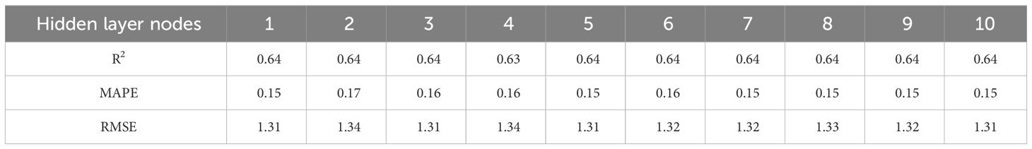
Table 1 R², MAPE and RMSE of the measured and predicted values of training samples with different hidden layer nodes.

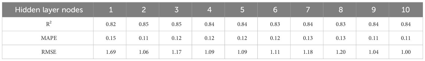
Table 2 R², MAPE and RMSE of the measured and predicted values of testing samples with different hidden layer nodes.

2.4.2 Random Forest

Random Forest (RF) is a powerful machine learning algorithm. As an ensemble learning technique, RF uses several decision trees, each of which is trained using randomly chosen feature and sample subsets (Belgiu and Drăguţ, 2016; Wang et al., 2023a). By averaging or voting the predictions from each individual tree, the final prediction is obtained (Belgiu and Drăguţ, 2016; Wang et al., 2023a). This study utilized the “TreeBagger” tool in MATLAB R2018a to construct a random forest model. Through experiment (Figure 2), the optimal number of trees and optimal number of leaf nodes were determined to be 200 and 5, respectively.

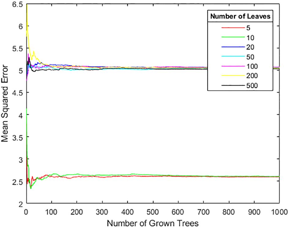
Figure 2 Determination of the optimal number of leaf nodes and trees.

2.4.3 Multiple Linear Regression

Multiple Linear Regression (MLR) describes how the dependent variable changes with multiple independent variables. This algorithm is simple, fast, low computational complexity, and suitable for local scale, widely used in remote sensing estimation of water parameters (Qing et al., 2013; Olmanson et al., 2016; Yang et al., 2017). This study used δ¹⁵N_PN as the dependent variable and optical indicators composed of remote sensing reflectance as the independent variable for multiple linear regression fitting. The fitting tool was the “regress” function in MATLAB R2018a software.

2.5 Accuracy evaluation

The accuracy evaluation of this study mainly includes four indices. Specific calculation formula of Pearson correlation coefficient (r), determination coefficient (R²), mean absolute percentage error (MAPE) and root mean square error (RMSE) are following Equations 2–5:

where n is the number of samples, ${\text{X}}_{\text{i}}$ and ${\text{Y}}_{\text{i}}$ refer to the value of two variables, Z and W denote the mean value of two variables in the sample.

3 Results

3.1 In situ distribution of TSM and Chl a concentration

As is shown in Figure 3, the TSM concentration ranged from 5.25 to 45.35 mg/L (averaged at 13.70 mg/L) in May. It should be noted that operational errors prevented us from obtaining the Chl a concentration outside the bay in May. Chl a concentration inside the bay ranged from 0.68 to 19.33 μg/L (averaged at 5.49 μg/L) in May. While in September, the concentration of TSM and Chl a ranged from 2.60 to 62.40 mg/L (with an average of 11.63 mg/L) and from 1.62 to 21.88 μg/L (with an average of 7.53 μg/L), respectively (Figure 3).

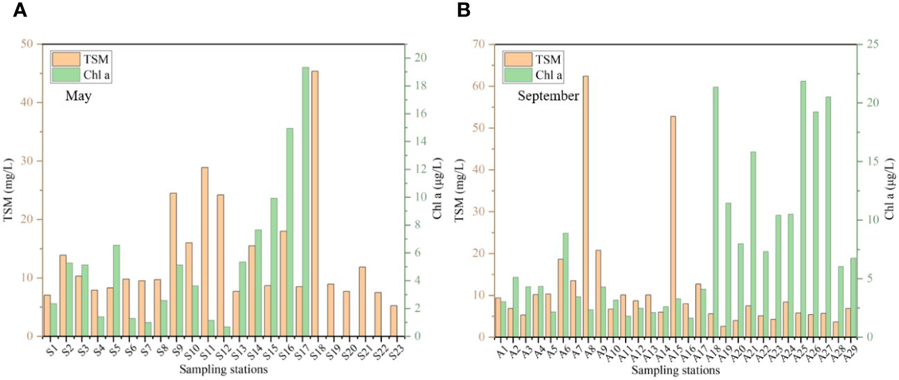
Figure 3 In situ distribution of the TSM and Chl a concentration in (A) May and (B) September.

3.2 In situ distribution of δ¹⁵N_PN and PN concentration

During the survey period, PN concentration ranged from 0.026 to 0.135 mg/L in May, with an average value of 0.048 mg/L. In September, PN concentration ranged from 0.022 to 0.09 mg/L, with an average value of 0.043 mg/L. Overall, the PN concentration in September was slightly lower than that in May. In addition, as shown in Figure 4, the average concentration of PN outside the bay was higher than that inside the bay in May and September. In May, the average concentration of PN outside and inside the bay was 0.062mg/L and 0.044mg/L, respectively. In September, the average concentration of PN outside and inside the bay was 0.053mg/L and 0.034mg/L, respectively. The δ¹⁵N value ranged from 5.89‰ to 10.14‰ (average 7.77‰) in May and 3.73‰ to 12.08‰ (average 7.77‰) in September, respectively. Similar to the distribution of PN concentration, the average δ¹⁵N outside the bay was higher than that inside the bay in May and September. Figure 4 presents that the average value of δ¹⁵N outside and inside the bay in May was 8.71% and 7.43%, respectively. In September, the average value of δ¹⁵N outside and inside the bay was 10% and 5.9%, respectively. The spatial distribution differences of δ¹⁵N inside and outside the bay were more pronounced in September (Figure 4).

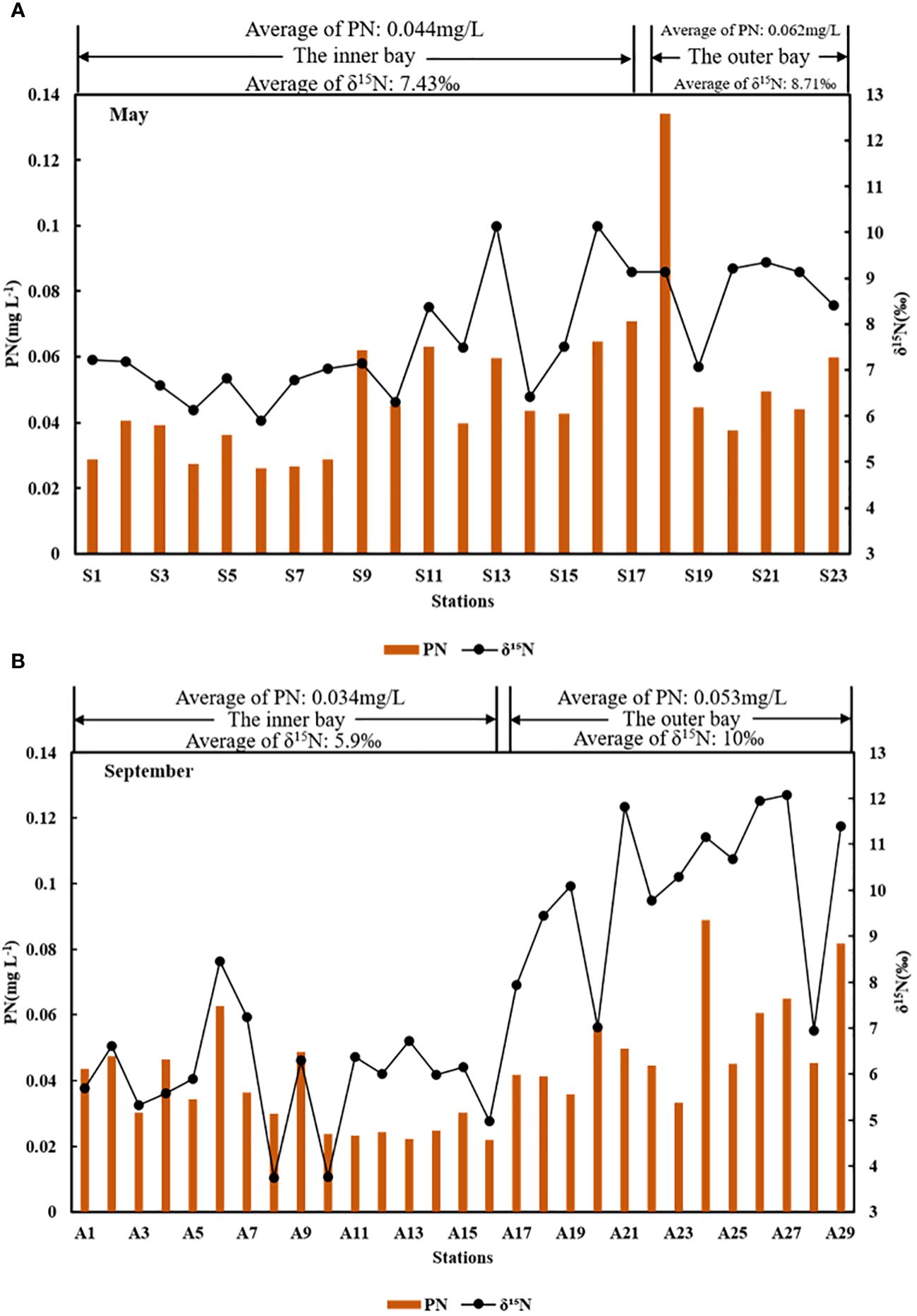
Figure 4 In situ distribution of the δ¹⁵N_PN and PN concentration in (A) May and (B) September.

3.3 Development, validation, and application of δ¹⁵N_PN retrieval model

Firstly, we conducted correlation analysis using in situ R_rs(λ) and δ¹⁵N_PN, and found that single band remote sensing reflectance retrieval was not effective, with low correlations (P>0.05), which will not be presented here. In order to obtain the best band combination of retrieval bands, we designed 6 optical indicators (Table 3). The method of optical indicators refers to the R_rs(λ) combination forms designed by Ling et al (Ling et al., 2020). Concretely, 240 possible combinations of R_rs(λ) with the sixteen OLCI bands (400 nm, 413 nm, 443 nm, 490 nm, 510 nm, 560 nm, 620 nm, 665 nm, 674 nm, 681 nm, 709 nm, 754 nm, 761 nm, 764 nm, 768 nm, and 779 nm) were trained by using MATLAB R2018a software to determine those optimal results for each form, X. After training, based on the correlation coefficient (r) between X and δ¹⁵N_PN, the highest value was taken, and the selection of λ₁ and λ₂ was ultimately determined (Table 3). From Table 3, it can be seen that X2 and X5 perform well, with r values of -0.78 (P<0.01) and -0.77 (P<0.01), respectively. We selected these two optical indicators as input variables for the model to construct δ¹⁵N_PN retrieval model.

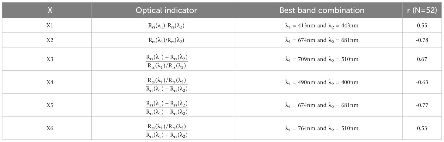
Table 3 Design of optical indicators and selection of optimal band combinations.

We randomly divided the dataset (input and output variables) into a training set (35 samples) and a testing set (17 samples), trained the model separately, and verified its performance. As shown in Figure 5, from the evaluation indices R², MAPE, and RMSE (Figure 5A-F), BPNN, RF and MLR methods perform well on the training sets (BPNN: R^2 = 0.64, MAPE = 14.93%, RMSE = 1.32‰; RF: R^2 = 0.70, MAPE = 13.84%, RMSE = 1.20‰; MLR: R^2 = 0.65, MAPE = 15.14%, RMSE = 1.29‰) and testing sets (BPNN: R^2 = 0.84, MAPE = 10.71%, RMSE = 0.99‰; RF: R^2 = 0.65, MAPE = 13.66%, RMSE = 1.22‰; MLR: R^2 = 0.84, MAPE = 11.94%, RMSE = 1.03‰), which can meet our retrieval requirements for δ¹⁵N_PN. To further validate the performance of BPNN, RF and MLR methods for δ¹⁵N_PN retrieval, we obtained quasi-synchronous Sentinel-3 data (September 20, 2016) during the sampling period, and obtained 20 satellite-ground matching points that were less affected by clouds, shadows, and solar flares. The established BPNN, RF and MLR models were applied to Sentinel-3 data. As shown in Figure 6, the BPNN and MLR model (BPNN: R^2 = 0.63, MAPE = 20.10%, RMSE = 1.63‰; MLR: R^2 = 0.63, MAPE = 20.71%, RMSE = 1.63‰) perform slightly better than the RF model (R^2 = 0.55, MAPE = 21.99%, RMSE = 1.67‰), with points more evenly distributed on both sides of the trend line. From Figure 6, it can be seen that the overall accuracy of the BPNN model is comparable to that of the MLR model, but the MAPE of BPNN model is slightly lower than that of the MLR model. Therefore, we used the BPNN model as the model for retrieving δ¹⁵N_PN. It is worth noting that there is a certain degree of overestimation or underestimation of satellite retrieval value of δ¹⁵N_PN (Figure 6). This may be due to the fact that the sampling time and satellite transit time are not synchronized in real-time (exceeding 24 hours), and the time window is an important factor affecting the accuracy of retrieval (Fu et al., 2023). On the other hand, it may be due to errors caused by atmospheric correction (Zhao et al., 2022). Moreover, Figure 7 shows the comparison between the OLCI-derived values of optical indicators (X2 and X5) and the measured values, demonstrating acceptable performance. The band combination reduces the errors caused by atmospheric correction in the algorithm implementation process to some extent (Zhao et al., 2022).

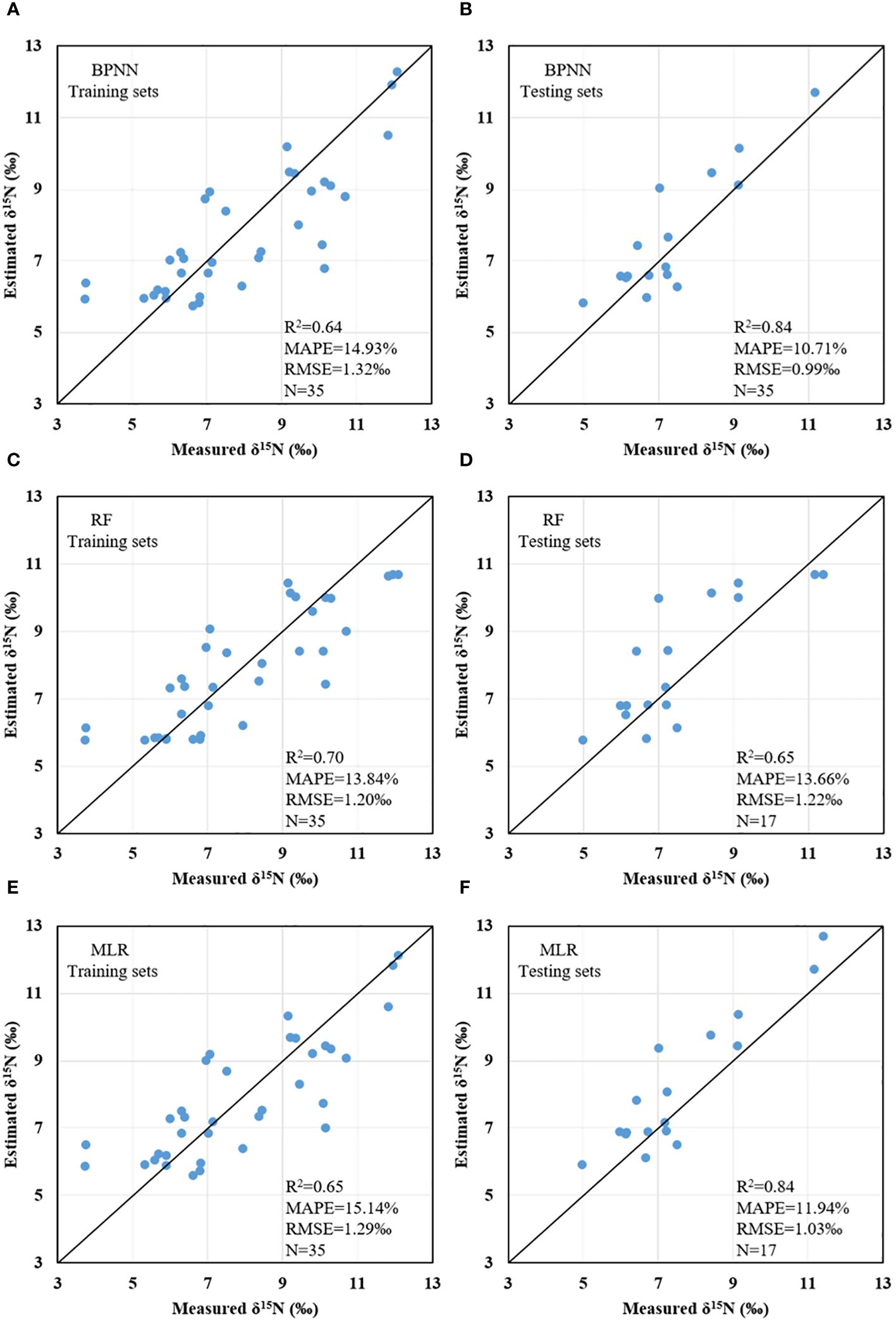
Figure 5 Scatter plots between the estimated δ¹⁵N_PN of BPNN (A, B), RF (C, D), and MLR (E, F) models and the measured δ¹⁵N_PN.

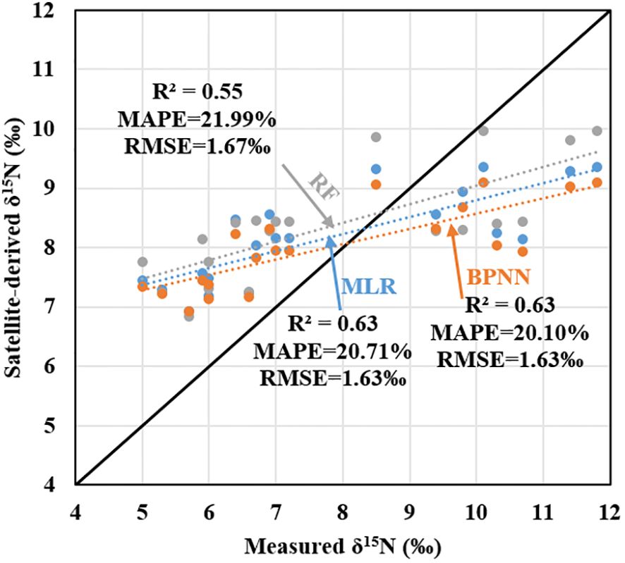
Figure 6 Scatter plots between the satellite-retrieved δ¹⁵N_PN using BPNN, RF and MLR models and the measured δ¹⁵N_PN in September 2016.

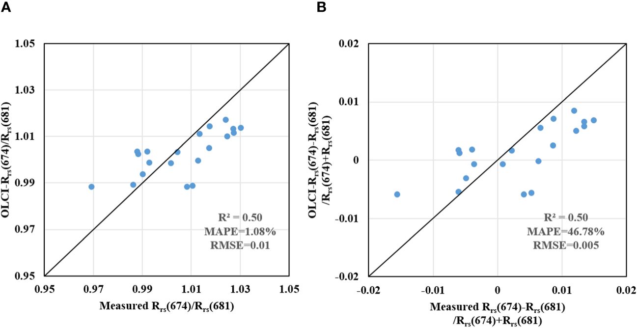
Figure 7 Comparison of measured and OLCI-derived values for match-up points at (A) R_rs(674)/R_rs(681) and (B) R_rs(674)-R_rs(681)/R_rs(674)+R_rs(681).

As shown in Figure 8, the spatial distribution map obtained by applying the BPNN model to Sentinel-3 data shows that δ¹⁵N_PN outside Zhanjiang Bay is slightly higher than inside Zhanjiang Bay. However, a few areas affected by factories, docks, and aquaculture areas (circled in Figure 8) (Lu et al., 2020; Zhang et al., 2020a; Zhou et al., 2022), these areas are highly susceptible to the influence of sewage or wastewater, resulting in higher dynamic changes in δ¹⁵N_PN in these areas. Therefore, the δ¹⁵N_PN retrieval results in these regions may have some differences from the measured values. But overall, the retrieval results are relatively consistent with the measured results, which also indicates that the BPNN model has a certain reliability in retrieving δ¹⁵N_PN. Simultaneously utilizing Sentinel-3 data to retrieve δ¹⁵N_PN has great potential for application.

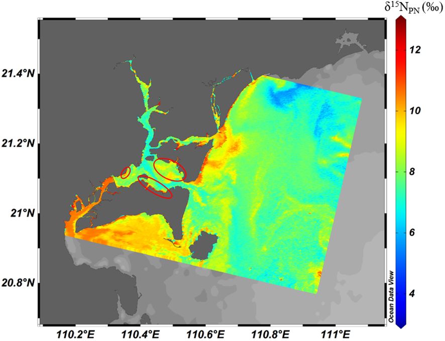
Figure 8 δ¹⁵N_PN retrieved from Sentinel-3 OLCI image (20 September 2016) in Zhanjiang Bay and its adjacent waters.

4 Discussion

4.1 Influencing factors of δ¹⁵N_PN and PN concentration

PN concentration and δ¹⁵N_PN in the ocean are influenced by various processes such as water mass mixing, nutrient gain and loss, and phytoplankton production (Sigman and Casciotti, 2001; Dagg et al., 2004; Ye et al., 2017). For bays strongly affected by human activities, PN concentration and δ¹⁵N_PN will also be affected by terrestrial factors such as soil, land runoff, and discharge of wastewater (Cloern et al., 2002; Bristow et al., 2013; Ye et al., 2017). Under the joint action of multiple factors, PN concentration and δ¹⁵N_PN in Zhanjiang Bay exhibited different characteristics in different months and regions.

TSM is the main carrier of terrestrial particulate matter (Chester and Jickells, 2012). As shown in Figure 9, there was a significant positive correlation between PN concentration and TSM concentration in May (r=0.746, P<0.01), but there was no significant correlation between PN concentration and TSM concentration in September. This indicated that terrestrial particulate matter in May had an important impact on PN concentration, while the terrestrial component content of PN in September was relatively low. To a certain extent, the Chl a concentration reflects the status of phytoplankton production (Luhtala et al., 2013). As illustrated in Figure 9, there was a certain positive correlation between PN concentration and Chl a concentration in May and September (r=0.647, P<0.01 for May; r=0.476, P<0.01 for September), indicating that phytoplankton production had a certain impact on PN concentration. In general, δ¹⁵N_PN can effectively indicate the source of PN (Ye et al., 2017; Chen et al., 2021). The δ¹⁵N_PN composition of marine organic matter range from 3‰ to 12‰ (Chen et al., 2021; Huang et al., 2021), while wastewater and livestock usually have the δ¹⁵N_PN values of 10‰ to 22‰ (Huang et al., 2021). The δ¹⁵N values ranged from 3.73‰ to 12.08‰ (average 7.77‰) in this study. Therefore, the source of PN in Zhanjiang Bay may be mainly marine organic matter, but terrestrial input was also mixed in, such as wastewater. In addition, there was a significant correlation between δ¹⁵N_PN and Chl a concentration in May and September (r=0.574, P<0.05 for May; r=0.806, P<0.01 for September; Figure 9). Both PN concentration and δ¹⁵N_PN showed a good correlation with Chl a concentration, indicating that phytoplankton production had a significant contribution to the source of PN.

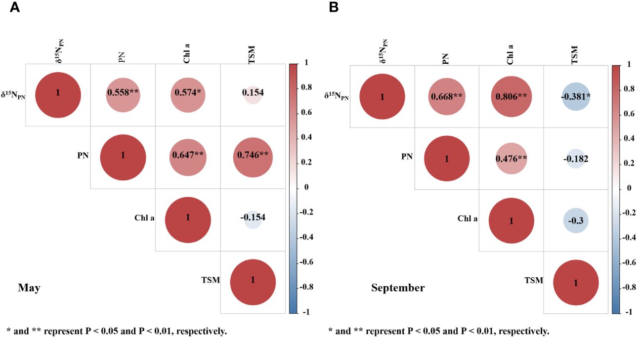
Figure 9 Correlation of PN concentration, δ¹⁵N_PN and related environmental parameters in the surface water of Zhanjiang Bay in May (A) and September (B).

Significantly, stations with higher δ¹⁵N_PN (>10 ‰) generally had higher Chl a concentration (>10 μg/L) (Table 4). The reception of hypereutrophic municipal wastewater in the bay area can easily lead to the bloom of phytoplankton, resulting in higher concentrations of Chl a (Gao et al., 2021). When the growth rate of phytoplankton accelerates, the isotopic fractionation that occurs during the rapid absorption of inorganic nitrogen by phytoplankton can lead to a heavier nitrogen isotope composition of particulate organic matter (Mariotti et al., 1984). Due to the preferential absorption of NH₄⁺ during the growth process of phytoplankton, the strong nitrification in coastal water and the preferential utilization of ¹⁴N in NH₄⁺ by phytoplankton can lead to the accumulation of residual NH₄⁺ in water by ¹⁵N (Cifuentes et al., 1988). When phytoplankton continue to absorb these enriched ¹⁵N in NH₄⁺, it will cause an increase in the δ¹⁵N_PN value of the produced particulate organic matter (Cifuentes et al., 1988; Ke et al., 2017). Moreover, due to the rapid economic development and increased human activities in Zhanjiang, the process of heterotrophic bacteria has been intensified (Li et al., 2021). The strong biodegradation process prioritizes the degradation of organic matter containing lighter isotopes, leading to the enrichment of residual organic matter with heavy nitrogen isotopes (Li et al., 2021). It is worth noting that the δ¹⁵N_PN value at station S13 and A29 was relatively high (>10 ‰), but the Chl a concentration was not high (5.34 μg/L and 6.75 μg/L, respectively), this may be due to the impact of sewage or wastewater input, as S13 and A29 are located near the factory and aquaculture industry, respectively. Previous study showed that in the region of algal uptake, sewage-derived NH₄⁺ and sewage-derived NO₃^- could raise the δ¹⁵N_PN value by 9.0-17.2‰ and 10-15‰, respectively (Estep and Vigg, 1985; Leavitt et al., 2006). In addition, Zhou et al. (2021) also indicated that during non-typhoon periods in Zhanjiang Bay, the PN heavy isotopes can be attributed to the utilization of mineralized NH₄⁺ from wastewater by phytoplankton. Therefore, the relatively heavy δ¹⁵N_PN component in Zhanjiang Bay and its adjacent waters can be attributed to phytoplankton production and sewage or wastewater input.

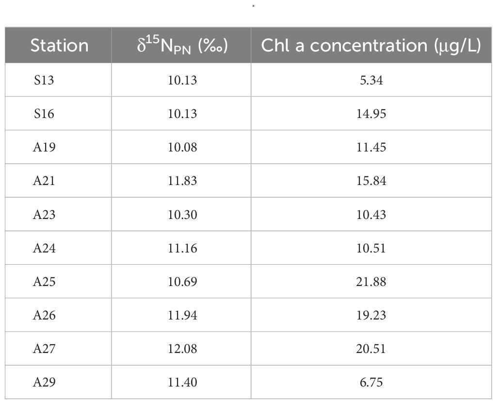
Table 4 Stations with higher δ¹⁵N_PN.

4.2 Evaluation of δ¹⁵N_PN remote sensing retrieval model

In section 4.1, we obtained that the PN source in Zhanjiang Bay is mainly phytoplankton production, and δ¹⁵N_PN had a good correlation with concentration of Chl a. Therefore, the δ¹⁵N_PN can be linked to the water color parameter Chl a, which can establish a suitable δ¹⁵N_PN remote sensing retrieval model. It is well-known that there is an absorption peak in the spectral reflectance near the wavelength of 674 nm due to the absorption of phytoplankton pigments, while there is a fluorescence peak near the wavelength of 681 nm, both of which are spectral characteristic bands specific to Chl a (Su et al., 2021). Consequently, choosing these two bands to retrieve δ¹⁵N_PN has a certain scientificity and reliability. In the RF model, due to the dominance of measured values between 5 and 11 in the training dataset, there may be biases in the decision tree constructed by decision tree learners, resulting in predicted values being concentrated within the range of 5 to 11. In addition, during prediction, each tree is given a predicted value, and the average of all predicted values is taken. This results in the predicted value of the random forest being within the range of the training sample’s predicted values, so it cannot be extrapolated. The predicted value can only be between the minimum and maximum values of the training sample’s predicted values, resulting in a set of identical estimated values between 10 and 11 in the testing set. When we need to infer independent or non independent variables that are beyond the range, the random forest does not do well (Wang et al., 2023b). The solution is to expand the scope of the dataset in the future to maintain balance. The BPNN model and MLR model performed well on both the training and testing sets, and they also performed well in the application of Sentinel-3 data. Although the multiple linear regression algorithm is simple and ease of implement, it should be noted that the regression coefficients of this model is only suitable for the Zhanjiang Bay and its adjacent sea areas. For other sea areas, parameter regionalization may be required, and the applicability of the model needs further verification. The samples in this study were collected during the rainy season. During the rainy season, increased rainfall leads to an increase in nutrients carried into the sea by land runoff, resulting in an increase in phytoplankton biomass (Baek et al., 2009). There was a good correlation between Chl a, and δ¹⁵N_PN in May and September. This provides a good foundation for the establishment of δ¹⁵N_PN remote sensing model. However, during the dry season, the decrease in rainfall leads to changes in the physical, chemical, and biological conditions of the water, as well as changes in the activity of phytoplankton. Whether Chl a and δ¹⁵N_PN still maintain a good correlation remains to be further explored. Whether the δ¹⁵N_PN retrieval model we established is still applicable depends on further sample collection and verification.

In order to better evaluate the δ¹⁵N_PN remote sensing retrieval model established in this study, we selected six widely used Chl a retrieval algorithms (Table 5), including 3 empirical algorithms (Three-band algorithm: TBA; Fluorescence Line Height algorithm:FLH; Maximum Chlorophyll Index algorithm: MCI) (Gower et al., 1999; Dall'Olmo et al., 2005; Gower et al., 2005) and 3 semi-analytical algorithms (Gons; Simis; Quasi-Analytical Algorithm improved form: QAA750E) (Gons et al., 2002; Simis et al., 2005; Xue et al., 2019), to attempt to retrieve δ¹⁵N_PN. As shown in Table 5, we substituted the in situ remote sensing reflectance into the expressions of the following six algorithms, and then perform comparison analysis between the results of the expressions with measured δ¹⁵N_PN. It is worth mentioning that the comparison analysis between the absorption coefficient of phytoplankton (a_ph(λ)) obtained by the semi-analytical algorithm and δ¹⁵N_PN was conducted. From Table 5, it can be seen that the BPNN algorithm proposed in this study has the highest accuracy (R^2 = 0.66, MAPE=13.52%, RMSE=1.19‰), followed by the TBA algorithm (R^2 = 0.49, MAPE=14.32%, RMSE=1.46‰). The Gons and Simis semi-analytical algorithms also have a good performance (Gons: R^2 = 0.46, MAPE=16.31%, RMSE=1.49‰; Simis: R^2 = 0.42, MAPE=16.81%, RMSE=1.56‰), indicating that semi-analytical algorithms have certain application potential in retrieving δ¹⁵N_PN. In addition, MCI algorithm, FLH algorithm and QAA750E algorithm perform poorly. Therefore, the algorithms composed of more bands may lead to more indeterminacy factors introduced, which directly affects the retrieval accuracy.

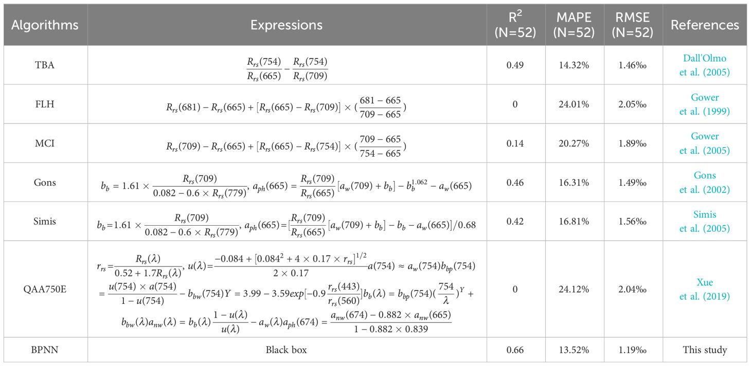
Table 5 Expressions of 6 Chl a retrieval algorithms and the comparison analysis between algorithm results and δ¹⁵N_PN..

Additionally, we obtained 18 measured δ¹⁵N_PN values in September 2017 and applied the BPNN model established in this study to the Sentinel-3 OLCI image data (18 September 2017). The retrieval results were shown in Figure 10. From the perspective of retrieval accuracy (Figure 11), the R², RMSE and MAPE were 0.59, 1.78‰, and 34.06%, respectively. The retrieval results can meet the requirements to a certain extent, indicating that our δ¹⁵N_PN retrieval model has certain applicability.

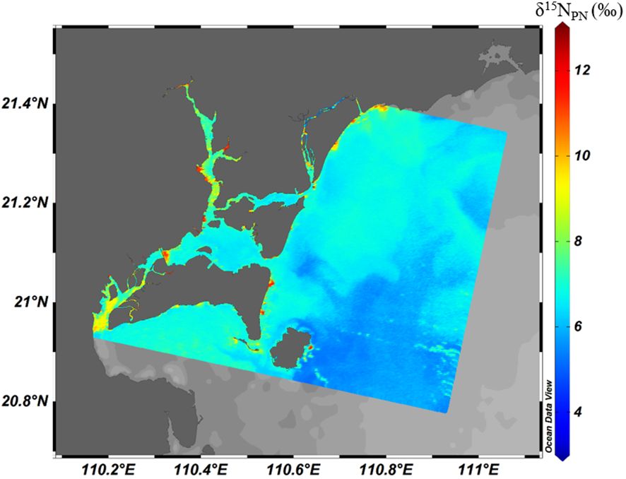
Figure 10 δ¹⁵N_PN retrieved from Sentinel-3 OLCI image (18 September 2017) in Zhanjiang Bay and its adjacent waters.

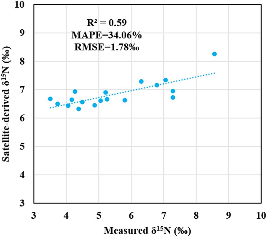
Figure 11 Scatter plots between the satellite-retrieved δ¹⁵N_PN using BPNN model and the measured δ¹⁵N_PN in September 2017.

4.3 The advantages and prospects of developing δ¹⁵N_PN remote sensing model

Isotope fractionation gives PN from different sources specific nitrogen stable isotope characteristic values, which provides the possibility of determining the source and destination of PN, making δ¹⁵N_PN a valuable tracer for tracking PN sources and understanding N cycling in water systems (Chen et al., 2021; Huang et al., 2021; Lu et al., 2021). Although traditional field surveys and chemical methods can accurately obtain δ¹⁵N_PN, they consume a lot of time, manpower, and resources. How to improve efficiency and enable us to quickly and extensively understand the dynamic changes of δ¹⁵N_PN? Satellite remote sensing has developed rapidly in recent decades, and various high-performance sensors have been developed for marine environmental monitoring, which is very conducive to our research and exploration of the ocean. Satellite remote sensing has irreplaceable advantages in large-scale spatial and long-term series monitoring. We only need to sacrifice a small amount of accuracy to obtain acceptable results, which is of great significance for the biogeochemical processes and nitrogen cycling research of PN in the ocean. According to the analysis above, water environmental pollution can also be distinguished by δ¹⁵N_PN values, which can indirectly indicate the pollution level of water bodies. This also provides a new method and strategy for traditional water quality monitoring and management.

However, the δ¹⁵N_PN remote sensing model established in this study only involves data from two cruises, and it cannot be denied that the limitations of the model exist. Meanwhile, the quality of satellite images and atmospheric correction can also bring uncertainty to δ¹⁵N_PN estimation. In the future, we will increase the sampling frequency and use more data from different seasons and regions to validate our established model, enhancing its robustness and universality.

5 Conclusions

Based on the measured δ¹⁵N_PN values and remote sensing reflectance in Zhanjiang Bay in May and September 2016, this study constructed three machine learning models (BPNN, RF, MLR) for δ¹⁵N_PN retrieval. After screening and analysis, the model input variables consisted of two optical indicators, namely R_rs(674)/R_rs(681) and $\frac{{\text{R}}_{\text{rs}}(674)-{\text{R}}_{\text{rs}}(681)}{{\text{R}}_{\text{rs}}(674)+{\text{R}}_{\text{rs}}(681)}$. Through the accuracy evaluation of the training sets and test sets and the analysis of the retrieval results of Sentinel-3, it was found that the BPNN model performed better compared to the other two models. In addition, PN source in Zhanjiang Bay was mainly phytoplankton production, and phytoplankton production was closely related to chlorophyll a, which provided a reliable basis for remote sensing retrieval of δ¹⁵N_PN. This basis was also confirmed by the fact that the two sensitive bands (674 nm and 681 nm) that respond to δ¹⁵N_PN were also the spectral characteristic bands of chlorophyll a. However, due to limited data sets and insufficient model optimization, the performance of the δ¹⁵N_PN retrieval model that we established still needs to be improved. In the future, we will continue to expand the data sets, optimize the model input variables, and construct a more robust δ¹⁵N_PN retrieval model for continuous and long-term monitoring.

Data availability statement

The raw data supporting the conclusions of this article will be made available by the authors, without undue reservation.

Author contributions

GY: Conceptualization, Investigation, Methodology, Software, Writing – original draft, Writing – review & editing. YZ: Conceptualization, Data curation, Formal analysis, Validation, Writing – review & editing. DF: Funding acquisition, Project administration, Supervision, Writing – review & editing. FC: Resources, Visualization, Writing – review & editing. CC: Methodology, Writing – review & editing.

Funding

The author(s) declare that financial support was received for the research, authorship, and/or publication of this article. This study was supported by the National Key Research and Development Program of China (No. 2022YFC3103101); Key Special Project for Introduced Talents Team of Southern Marine Science and Engineering Guangdong Laboratory (No. GML2021GD0809); National Natural Science Foundation of China (No. 42206187); Key projects of the Guangdong Education Department (No. 2023ZDZX4009).

Conflict of interest

The authors declare that the research was conducted in the absence of any commercial or financial relationships that could be construed as a potential conflict of interest.

Publisher’s note

All claims expressed in this article are solely those of the authors and do not necessarily represent those of their affiliated organizations, or those of the publisher, the editors and the reviewers. Any product that may be evaluated in this article, or claim that may be made by its manufacturer, is not guaranteed or endorsed by the publisher.

References

Baek S. H., Shimode S., Kim H. C., Han M. S., Kikuchi T. (2009). Strong bottom-up effects on phytoplankton community caused by a rainfall during spring and summer in Sagami Bay, Japan. J. Mar. Syst. 75, 253–264. doi: 10.1016/j.jmarsys.2008.10.005
Belgiu M., Drăguţ L. (2016). Random forest in remote sensing: A review of applications and future directions. ISPRS J. Photogramm. Remote Sens. 114, 24–31. doi: 10.1016/j.isprsjprs.2016.01.011
Bristow L. A., Jickells T. D., Weston K., Marca-Bell A., Parker R., Andrews J. E. (2013). Tracing estuarine organic matter sources into the southern North Sea using C and N isotopic signatures. Biogeochemistry 113, 9–22. doi: 10.1007/s10533-012-9758-4
Cao Z., Ma R., Duan H., Pahlevan N., Melack J., Shen M., et al. (2020). A machine learning approach to estimate chlorophyll-a from Landsat-8 measurements in inland lakes. Remote Sens. Environ. 248, 111974. doi: 10.1016/j.rse.2020.111974
Capone D. G., Bronk D. A., Mulholland M. R., Carpenter E. J. (2008). Nitrogen in the marine environment (Amsterdam: Elsevier), 1–50.
Chen F., Lao Q., Jia G., Chen C., Zhu Q., Zhou X. (2019). Seasonal variations of nitrate dual isotopes in wet deposition in a tropical city in China. Atmos. Environ. 196, 1–9. doi: 10.1016/j.atmosenv.2018.09.061
Chen F., Lu X., Song Z., Huang C., Jin G., Chen C., et al. (2021). Coastal currents regulate the distribution of the particulate organic matter in western Guangdong offshore waters as evidenced by carbon and nitrogen isotopes. Mar. pollut. Bull. 172, 112856. doi: 10.1016/j.marpolbul.2021.112856
Chen J., Quan W., Cui T., Song Q. (2015). Estimation of total suspended matter concentration from MODIS data using a neural network model in the China eastern coastal zone. Estuar. Coast. Shelf Sci. 155, 104–113. doi: 10.1016/j.ecss.2015.01.018
Cifuentes L. A., Sharp J. H., Fogel M. L. (1988). Stable carbon and nitrogen isotope biogeochemistry in the Delaware estuary. Limnol. Oceanogr. 33, 1102–1115. doi: 10.4319/lo.1988.33.5.1102
Cloern J. E., Canuel E. A., Harris D. (2002). Stable carbon and nitrogen isotope composition of aquatic and terrestrial plants of the San Francisco Bay estuarine system. Limnol. Oceanogr. 47, 713–729. doi: 10.4319/lo.2002.47.3.0713
Dagg M., Benner R., Lohrenz S., Lawrence D. (2004). Transformation of dissolved and particulate materials on continental shelves influenced by large rivers: plume processes. Cont. Shelf Res. 24, 833–858. doi: 10.1016/j.csr.2004.02.003
Dall'Olmo G., Gitelson A. A., Rundquist D. C., Leavitt B., Barrow T., Holz J. C. (2005). Assessing the potential of SeaWiFS and MODIS for estimating chlorophyll concentration in turbid productive waters using red and near-infrared bands. Remote Sens. Environ. 96, 176–187. doi: 10.1016/j.rse.2005.02.007
Du C., Wang Q., Li Y., Lyu H., Zhu L., Zheng Z., et al. (2018). Estimation of total phosphorus concentration using a water classification method in inland water. Int. J. Appl. Earth Obs. Geoinf. 71, 29–42. doi: 10.1016/j.jag.2018.05.007
Eppley R. W., Peterson B. J. (1979). Particulate organic matter flux and planktonic new production in the deep ocean. Nature 282, 677–680. doi: 10.1038/282677a0
Estep M. L., Vigg S. (1985). Stable carbon and nitrogen isotope tracers of trophic dynamics in natural populations and fisheries of the Lahontan Lake system, Nevada. Can. J. Fish. Aquat.Sci. 42, 1712–1719. doi: 10.1139/f85-215
Falkowski P. G. (1997). Evolution of the nitrogen cycle and its influence on the biological sequestration of CO2 in the ocean. Nature 387, 272–275. doi: 10.1038/387272a0
Fu L., Zhou Y., Liu G., Song K., Tao H., Zhao F., et al. (2023). Retrieval of chla concentrations in lake Xingkai using OLCI images. Remote Sens. 15, 3809. doi: 10.3390/rs15153809
Galloway J. N., Dentener F. J., Capone D. G., Boyer E. W., Howarth R. W., Seitzinger S. P., et al. (2004). Nitrogen cycles: past, present, and future. Biogeochemistry 70, 153–226. doi: 10.1007/s10533-004-0370-0
Gao C., Yu F., Chen J., Huang Z., Jiang Y., Zhuang Z., et al. (2021). Anthropogenic impact on the organic carbon sources, transport and distribution in a subtropical semi-enclosed bay. Sci. Total Environ. 767, 145047. doi: 10.1016/j.scitotenv.2021.145047
Gons H. J., Rijkeboer M., Ruddick K. G. (2002). A chlorophyll-retrieval algorithm for satellite imagery (Medium Resolution Imaging Spectrometer) of inland and coastal waters. J. Plankton Res. 24, 947–951. doi: 10.1093/plankt/24.9.947
Gower J. F. R., Doerffer R., Borstad G. A. (1999). Interpretation of the 685nm peak in water-leaving radiance spectra in terms of fluorescence, absorption and scattering, and its observation by MERIS. Int. J. Remote Sens. 20, 1771–1786. doi: 10.1080/014311699212470
Gower J., King S., Borstad G., Brown L. (2005). Detection of intense plankton blooms using the 709 nm band of the MERIS imaging spectrometer. Int. J. Remote Sens. 26, 2005–2012. doi: 10.1080/01431160500075857
Granger J., Sigman D. M., Rohde M. M., Maldonado M. T., Tortell P. D. (2010). N and O isotope effects during nitrate assimilation by unicellular prokaryotic and eukaryotic plankton cultures. Geochim. Cosmochim. Acta 74, 1030–1040. doi: 10.1016/j.gca.2009.10.044
Huang C., Chen F., Zhang S., Chen C., Meng Y., Zhu Q., et al. (2020). Carbon and nitrogen isotopic composition of particulate organic matter in the Pearl River Estuary and the adjacent shelf. Estuarine Coast. Shelf Sci. 246, 107003. doi: 10.1016/j.ecss.2020.107003
Huang C., Lao Q., Chen F., Zhang S., Chen C., Bian P., et al. (2021). Distribution and sources of particulate organic matter in the northern south China Sea: implications of human activity. J. Ocean Univ. China. 20, 1136–1146. doi: 10.1007/s11802-021-4807-z
Ju A., Wang H., Wang L., Weng Y. (2023). Application of machine learning algorithms for prediction of ultraviolet absorption spectra of chromophoric dissolved organic matter (CDOM) in seawater. Front. Mar. Sci. 10, 1065123. doi: 10.3389/fmars.2023.1065123
Ke Z., Tan Y., Huang L., Zhao C., Jiang X. (2017). Spatial distributions of δ13C, δ15N and C/N ratios in suspended particulate organic matter of a bay under serious anthropogenic influences: Daya Bay, China. Mar. pollut. Bull. 114, 183–191. doi: 10.1016/j.marpolbul.2016.08.078
Lao Q., Liu G., Shen Y., Su Q., Lei X. (2021). Biogeochemical processes and eutrophication status of nutrients in the northern Beibu Gulf, South China. J. Earth Syst. Sci. 130, 199. doi: 10.1007/s12040-021-01706-y
Leavitt P. R., Brock C. S., Ebel C., Patoine A. (2006). Landscape-scale effects of urban nitrogen on a chain of freshwater lakes in central North America. Limnol. Oceanogr. 51, 2262–2277. doi: 10.4319/lo.2006.51.5.2262
Li J., Chen F., Zhang S., Huang C., Chen C., Zhou F., et al. (2021). Origin of the particulate organic matter in a monsoon-controlled bay in southern China. J. Mar. Sci. Eng. 9, 541. doi: 10.3390/jmse9050541
Ling Z., Sun D., Wang S., Qiu Z., Huan Y., Mao Z., et al. (2020). Remote sensing estimation of colored dissolved organic matter (CDOM) from GOCI measurements in the Bohai Sea and Yellow Sea. Environ. Sci. pollut. Res. 27, 6872–6885. doi: 10.1007/s11356-019-07435-6
Liu H., Li Q., Bai Y., Yang C., Wang J., Zhou Q., et al. (2021). Improving satellite retrieval of oceanic particulate organic carbon concentrations using machine learning methods. Remote Sens. Environ. 256, 112316. doi: 10.1016/j.rse.2021.112316
Liu Y., Xu L., Li M. (2017). The parallelization of back propagation neural network in mapreduce and spark. Int. J. Parallel Progr. 45, 760–779. doi: 10.1007/s10766-016-0401-1
Lu X., Huang C., Chen F., Zhang S., Lao Q., Chen C., et al. (2021). Carbon and nitrogen isotopic compositions of particulate organic matter in the upwelling zone off the east coast of Hainan Island, China. Mar. pollut. Bull. 167, 112349. doi: 10.1016/j.marpolbul.2021.112349
Lu X., Zhou F., Chen F., Lao Q., Zhu Q., Meng Y., et al. (2020). Spatial and seasonal variations of sedimentary organic matter in a subtropical bay: Implication for human interventions. Int. J. Environ. Res. Public Health 17, 1362. doi: 10.3390/ijerph17041362
Luhtala H., Tolvanen H., Kalliola R. (2013). Annual spatio-temporal variation of the euphotic depth in the SW-Finnish archipelago, Baltic Sea. Oceanologia 55, 359–373. doi: 10.5697/oc.55-2.359
Maciel D. A., Barbosa C. C. F., de Moraes Novo E. M. L., Júnior R. F., Begliomini F. N. (2021). Water clarity in Brazilian water assessed using Sentinel-2 and machine learning methods. ISPRS J. Photogramm. Remote Sens. 182, 134–152. doi: 10.1016/j.isprsjprs.2021.10.009
MacKay D. J. (1992). Bayesian interpolation. Neural comput. 4, 415–447. doi: 10.1162/neco.1992.4.3.415
Mariotti A., Lancelot C., Billen G. (1984). Natural isotopic composition of nitrogen as a tracer of origin for suspended organic matter in the Scheldt estuary. Geochim. Cosmochim. Acta 48, 549–555. doi: 10.1016/0016-7037(84)90283-7
Mathew M. M., Srinivasa Rao N., Mandla V. R. (2017). Development of regression equation to study the Total Nitrogen, Total Phosphorus and Suspended Sediment using remote sensing data in Gujarat and Maharashtra coast of India. J. Coast. Conserv. 21, 917–927. doi: 10.1007/s11852-017-0561-1
Mobley C. D. (1999). Estimation of the remote-sensing reflectance from above-surface measurements. Appl. opt. 38, 7442–7455. doi: 10.1364/AO.38.007442
Montoya J. P., Carpenter E. J., Capone D. G. (2002). Nitrogen fixation and nitrogen isotope abundances in zooplankton of the oligotrophic North Atlantic. Limnol. Oceanogr. 47, 1617–1628. doi: 10.4319/lo.2002.47.6.1617
Olmanson L. G., Brezonik P. L., Finlay J. C., Bauer M. E. (2016). Comparison of Landsat 8 and Landsat 7 for regional measurements of CDOM and water clarity in lakes. Remote Sens. Environ. 185, 119–128. doi: 10.1016/j.rse.2016.01.007
Ondrusek M., Stengel E., Kinkade C. S., Vogel R. L., Keegstra P., Hunter C., et al. (2012). The development of a new optical total suspended matter algorithm for the Chesapeake Bay. Remote Sens. Environ. 119, 243–254. doi: 10.1016/j.rse.2011.12.018
Pahlevan N., Smith B., Schalles J., Binding C., Cao Z., Ma R., et al. (2020). Seamless retrievals of chlorophyll-a from Sentinel-2 (MSI) and Sentinel-3 (OLCI) in inland and coastal waters: A machine-learning approach. Remote Sens. Environ. 240, 111604. doi: 10.1016/j.rse.2019.111604
Pajares S., Ramos R. (2019). Processes and microorganisms involved in the marine nitrogen cycle: knowledge and gaps. Front. Mar. Sci. 6, 739. doi: 10.3389/fmars.2019.00739
Qing S., Zhang J., Cui T., Bao Y. (2013). Retrieval of sea surface salinity with MERIS and MODIS data in the Bohai Sea. Remote Sens. Environ. 136, 117–125. doi: 10.1016/j.rse.2013.04.016
Sarma V. V. S. S., Krishna M. S., Srinivas T. N. R. (2020). Sources of organic matter and tracing of nutrient pollution in the coastal Bay of Bengal. Mar. pollut. Bull. 159, 111477. doi: 10.1016/j.marpolbul.2020.111477
Shen M., Duan H., Cao Z., Xue K., Qi T., Ma J., et al. (2020). Sentinel-3 OLCI observations of water clarity in large lakes in eastern China: Implications for SDG 6.3. 2 evaluation. Remote Sens. Environ. 247, 111950. doi: 10.1016/j.rse.2020.111950
Shen M., Luo J., Cao Z., Xue K., Qi T., Ma J., et al. (2022). Random forest: An optimal chlorophyll-a algorithm for optically complex inland water suffering atmospheric correction uncertainties. J. Hydrol. 615, 128685. doi: 10.1016/j.jhydrol.2022.128685
Sigman D. M., Casciotti K. L. (2001). Nitrogen isotopes in the ocean (Amsterdam: Elsevier), 1884–1894. doi: 10.1006/rwos.2001.0172
Simis S. G., Peters S. W., Gons H. J. (2005). Remote sensing of the cyanobacterial pigment phycocyanin in turbid inland water. Limnol. Oceanogr. 50, 237–245. doi: 10.4319/lo.2005.50.1.0237
Su H., Lu X., Chen Z., Zhang H., Lu W., Wu W. (2021). Estimating coastal chlorophyll-a concentration from time-series OLCI data based on machine learning. Remote Sens. 13, 576. doi: 10.3390/rs13040576
Sun D., Li Y., Wang Q., Le C. (2009). Remote sensing retrieval of CDOM concentration in Lake Taihu with hyper-spectral data and neural network model. Geomatics Inf. Sci. Wuhan University. 34, 851–855.
Tian D., Zhao X., Gao L., Liang Z., Yang Z., Zhang P., et al. (2024). Estimation of water quality variables based on machine learning model and cluster analysis-based empirical model using multi-source remote sensing data in inland reservoirs, South China. Environ. pollut. 342, 123104. doi: 10.1016/j.envpol.2023.123104
Voss M., Bange H. W., Dippner J. W., Middelburg J. J., Montoya J. P., Ward B. (2013). The marine nitrogen cycle: recent discoveries, uncertainties and the potential relevance of climate change. Philos. Trans. R. Soc. B. 368, 20130121. doi: 10.1098/rstb.2013.0121
Wang Y., Liu H., Wu G. (2022). Satellite retrieval of oceanic particulate organic nitrogen concentration. Front. Mar. Sci. 9, 943867. doi: 10.3389/fmars.2022.943867
Wang J., Tang J., Wang W., Wang Y., Wang Z. (2023a). Quantitative retrieval of chlorophyll-a concentrations in the Bohai-yellow sea using GOCI surface reflectance products. Remote Sens. 15 (22), 5285. doi: 10.3390/rs15225285
Wang J., Wu X., Ma D., Wen J., Xiao Q. (2023b). Remote sensing retrieval based on machine learning algorithm: Uncertainty analysis. Natl. Remote Sens. Bullet. 27 (3), 790–801. doi: 10.11834/jrs.20221172
Watanabe F., Alcântara E., Curtarelli M., Kampel M., Stech J. (2018). Landsat-based remote sensing of the colored dissolved organic matter absorption coefficient in a tropical oligotrophic reservoir. Remote Sens. Appl.: Soc Environ. 9, 82–90. doi: 10.1016/j.rsase.2017.12.004
Wu Y., Dittmar T., Ludwichowski K. U., Kattner G., Zhang J., Zhu Z. Y., et al. (2007). Tracing suspended organic nitrogen from the Yangtze River catchment into the East China Sea. Mar. Chem. 107, 367–377. doi: 10.1016/j.marchem.2007.01.022
Xu Y., Zhang Y., Zhang D. (2010). Retrieval of dissolved inorganic nitrogen from multi-temporal MODIS data in Haizhou Bay. Mar. Geod. 33, 1–15. doi: 10.1080/01490410903530257
Xue K., Ma R., Duan H., Shen M., Boss E., Cao Z. (2019). Inversion of inherent optical properties in optically complex waters using sentinel-3A/OLCI images: A case study using China's three largest freshwater lakes. Remote Sens. Environ. 225, 328–346. doi: 10.1016/j.rse.2019.03.006
Yang Z., Reiter M., Munyei N. (2017). Estimation of chlorophyll-a concentrations in diverse water bodies using ratio-based NIR/Red indices. Remote Sens. Appl.: Soc Environ. 6, 52–58. doi: 10.1016/j.rsase.2017.04.004
Ye F., Guo W., Shi Z., Jia G., Wei G. (2017). Seasonal dynamics of particulate organic matter and its response to flooding in the Pearl River Estuary, China, revealed by stable isotope (δ13C and δ15N) analyses. J. Geophys. Res.: Oceans. 122, 6835–6856. doi: 10.1002/2017JC012931
Yu G., Zhong Y., Liu S., Lao Q., Chen C., Fu D., et al. (2023). Remote sensing estimates of particulate organic carbon sources in the Zhanjiang bay using sentinel-2 data and carbon isotopes. Remote Sens. 15, 3768. doi: 10.3390/rs15153768
Zhang J., Fu M., Zhang P., Sun D., Peng D. (2023). Unravelling nutrients and carbon interactions in an urban coastal water during algal bloom period in Zhanjiang bay, China. Water 15, 900. doi: 10.3390/w15050900
Zhang P., Peng C. H., Zhang J. B., Zou Z. B., Shi Y. Z., Zhao L. R., et al. (2020a). Spatiotemporal urea distribution, sources, and indication of DON bioavailability in Zhanjiang Bay, China. Water 12, 633. doi: 10.3390/w12030633
Zhang P., Xu J. L., Zhang J. B., Li J. X., Zhang Y. C., Li Y., et al. (2020b). Spatiotemporal dissolved silicate variation, sources, and behavior in the eutrophic Zhanjiang Bay, China. Water 12, 3586. doi: 10.3390/w12123586
Zhao Z., Cai X., Huang C., Shi K., Li J., Jin J., et al. (2022). A novel semianalytical remote sensing retrieval strategy and algorithm for particulate organic carbon in inland waters based on biogeochemical-optical mechanisms. Remote Sens. Environ. 280, 113213. doi: 10.1016/j.rse.2022.113213
Zheng H., Wu Y., Han H., Wang J., Liu S., Xu M., et al. (2024). Utilizing residual networks for remote sensing estimation of total nitrogen concentration in Shandong offshore areas. Front. Mar. Sci. 11, 1336259. doi: 10.3389/fmars.2024.1336259
Zhou X., Jin G., Li J., Song Z., Zhang S., Chen C., et al. (2021). Effects of typhoon mujigae on the biogeochemistry and ecology of a semi-enclosed bay in the northern South China sea. J. Geophys. Res.: Biogeosci. 126, e2020JG006031. doi: 10.1029/2020JG006031
Keywords: particulate nitrogen, δ15NPN, remote sensing, machine learning algorithm, Sentinel-3, OLCI, Zhanjiang Bay
Citation: Yu G, Zhong Y, Fu D, Chen F and Chen C (2024) Remote sensing estimation of δ15NPN in the Zhanjiang Bay using Sentinel-3 OLCI data based on machine learning algorithm. Front. Mar. Sci. 11:1366987. doi: 10.3389/fmars.2024.1366987
Received: 08 January 2024; Accepted: 24 April 2024;
Published: 14 May 2024.
Edited by:
Huizeng Liu, Shenzhen University, ChinaReviewed by:
Chenggong Du, Huaiyin Normal University, ChinaZhubin Zheng, Gannan Normal University, China
Copyright © 2024 Yu, Zhong, Fu, Chen and Chen. This is an open-access article distributed under the terms of the Creative Commons Attribution License (CC BY). The use, distribution or reproduction in other forums is permitted, provided the original author(s) and the copyright owner(s) are credited and that the original publication in this journal is cited, in accordance with accepted academic practice. No use, distribution or reproduction is permitted which does not comply with these terms.
*Correspondence: Yafeng Zhong, yiyi1372472@163.com; Dongyang Fu, fdy163@163.com