


Abstract
The Photometric objects Around Cosmic webs (PAC) approach developed in Xu et al. has the advantage of making full use of spectroscopic and deeper photometric surveys. With the merits of PAC, the excess surface density  of neighboring galaxies can be measured down to stellar mass 1010.80M⊙ around quasars at redshift 0.8 < zs < 1.0, with the data from the Sloan Digital Sky Survey IV extended Baryon Oscillation Spectroscopic Survey and the Dark Energy Spectroscopic Instrument Legacy Imaging Surveys. We find that
  generally increases quite steeply with the decrease of the separation. Using the subhalo abundance-matching method, we can accurately model the
  both on small and large scales. We show that the steep increase of
  toward the quasars requires that a large fraction
  of quasars should be satellites in massive halos, and we find that this fraction measurement is insensitive to the assumptions of our modeling. This high satellite fraction indicates that the subhalos have nearly the same probability of hosting quasars as the halos for the same (infall) halo mass and that the large-scale environment has negligible effect on the quasar activity. We show that even with this high satellite fraction, each massive halo on average does not host more than one satellite quasar, due to the sparsity of quasars.
Export citation and abstract BibTeX RIS

Original content from this work may be used under the terms of the Creative Commons Attribution 4.0 licence. Any further distribution of this work must maintain attribution to the author(s) and the title of the work, journal citation and DOI.
1. Introduction
The large-scale structure of the Universe is primarily influenced by dark matter that only undergoes gravitational interactions. Various luminous tracers, such as luminous red galaxies (LRGs), quasars, and emission-line galaxies, are employed to understand the distribution of the underlying dark matter. Quasars are the most luminous tracer among these and can reach high redshift (zs > 2.0), 5 offering invaluable information for investigating structure formation and cosmology in the early Universe (du Mas des Bourboux et al. 2020; Neveux et al. 2020; Hou et al. 2021; Brieden et al. 2022). Moreover, quasars are believed to be powered by the mass accretion onto supermassive black holes (SMBHs) located at the center of each galaxy (Soltan 1982). The strong feedback from the SMBHs regulates the formation of their host galaxies, shaping a process of co-evolution (Heckman & Best 2014). This underscores the importance of understanding quasars in the broader context of galaxy formation.
In the realm of both cosmological and galaxy formation studies employing quasars, it is crucial to accurately delineate the connection between quasars and the underlying dark matter, which often involves precise measurements of the number density and multiscale clustering of quasars. Since the pioneering work of Osmer (1981), extensive efforts have been dedicated to quantifying quasar clustering through correlation functions. Among these, the two-point correlation function (2PCF) stands out as the predominant method. The availability of data sets such as the 2dF Quasi-Stellar Object Redshift Survey (2QZ; Croom et al. 2004), the Sloan Digital Sky Survey (SDSS)-I/II/III/BOSS, and SDSS-IV/the extended Baryon Oscillation Spectroscopic Survey (eBOSS; Schneider et al. 2010, 2002; Eisenstein et al. 2011; Lyke et al. 2020), along with the emergence of surveys like the Dark Energy Spectroscopic Instrument (DESI) survey (DESI Collaboration et al. 2016), the Subaru Prime Focus Spectrograph survey (Tamura et al. 2018), and the Euclid survey (Laureijs et al. 2011), has enabled high-precision measurements of the 2PCF at large scales (>1 h−1 Mpc). However, accurately measuring quasar clustering at small scales (<1 h−1 Mpc) remains challenging, due to the technical issue of fiber collisions and the low quasar number density. While several upweighting schemes have been proposed to address the fiber collision problem (Jing et al. 1998; Guo et al. 2012; Reid et al. 2014; Hahn et al. 2017; Percival & Bianchi 2017; Yang et al. 2019; Sunayama et al. 2020), and additional observations have been conducted to increase the number of quasar pairs selected from 2QZ and SDSS images (Hennawi et al. 2006; Myers et al. 2008; Richardson et al. 2012; Eftekharzadeh et al. 2017), the inherent difficulties persist. Moreover, numerous studies seek to enhance small-scale measurements by cross-correlating quasars with other spectroscopic tracers, such as LRGs (Kauffmann & Haehnelt 2002; Padmanabhan et al. 2009; Miyaji et al. 2011; Shen et al. 2013; Zhang et al. 2013). Although small-scale measurements can be more precise than relying solely on quasar autocorrelation, the obstacles remain, as the the other tracers are also sparse at high redshift and the fiber collision issue may persist.
On the modeling front, various studies have aimed to establish connections between observed quasars and the underlying dark matter. In the simplest scenario, the linear bias factor can be determined by examining the relative amplitude of dark matter and quasars in the 2PCF at large scales (Jing 1998). This linear bias factor, in turn, can be employed to provide a rough estimate for the typical mass of the dark matter halos that host quasars (Ross et al. 2009). The halo occupation distribution (HOD) method has been utilized to model the 2PCF for an extensive range. Numerous studies have consistently found that the typical mass of quasars falls within the range of 1012 h−1 M⊙ ∼ 1013 h−1 M⊙, showing a remarkable degree of independence with respect to redshift or quasar luminosity (Porciani et al. 2004; Croom et al. 2005; Myers et al. 2006, 2007; Coil et al. 2007; Shen et al. 2007, 2013; da Ângela et al. 2008; Padmanabhan et al. 2009; Richardson et al. 2012; White et al. 2012; Mitra et al. 2018; Powell et al. 2020).
The satellite fraction of quasars can be derived using the HOD framework, and this measurement proves particularly sensitive to small-scale clustering. As noted previously, accurately measuring the small-scale clustering of quasars poses a challenge, leading to discrepant results in the literature (Starikova et al. 2011; Kayo & Oguri 2012; Leauthaud et al. 2015; Eftekharzadeh et al. 2019; Georgakakis et al. 2019; Alam et al. 2021). For instance, the satellite fraction of quasars is determined as  and
and  through the cross-correlation between quasars and LRGs under two distinct quasar HOD models at redshift 0.3–0.9 (Shen et al. 2013). Additionally, it is measured to be
  using the autocorrelation of quasars at redshift 0.4–2.5 (Richardson et al. 2012). However, it is important to determine this fraction, as the information is crucial not only for determining the small-scale clustering of quasars (e.g., the close pairs), but also for studying the halo environment effect on the formation of quasars.
In this study, to achieve precise measurements of quasar clustering across various scales and accurately constrain the quasar–halo connection and satellite fraction, we utilize the Photometric Objects Around Cosmic Webs (PAC) approach. On the basis of Wang et al. (2011), Xu et al. (2022b) developed the PAC method, which capitalizes on the benefits of leveraging both spectroscopic and deeper photometric surveys. PAC can measure the excess surface density  of photometric objects with specific physical properties around spectroscopic tracers. With the PAC method, Xu et al. (2022a, 2023) precisely determined the stellar–halo mass relation (SHMR) and galaxy stellar mass function down to the stellar mass limit where the spectroscopic sample is already highly incomplete, emphasizing the effectiveness of the PAC method. Given the absence of fiber collision problems between photometric and spectroscopic surveys, PAC becomes a valuable tool for accurately measuring the environment on the h−1 Mpc scale for quasars. Additionally, PAC enables the assessment of the spatial distribution of galaxies with diverse properties around quasars, offering extensive information to study the quasar–halo connection. We use the quasar sample from the Sixteenth Data Release (DR16) of SDSS-IV/eBOSS (Prakash et al. 2016; Ahumada et al. 2020; Lyke et al. 2020) and the photometric sample from the Ninth Data release (DR9) of the DESI Legacy Imaging Surveys (Legacy Surveys; Dey et al. 2019). We concentrate on a limited redshift range of 0.8 < zs < 1.0, due to constraints posed by the survey depth of the Legacy Surveys. We employ the subhalo abundance-matching method (SHAM) to model the
  measurements from PAC and simultaneously constrain the SHMR for galaxies and the quasar–halo connection. Our analysis of the quasar–halo connection reveals a substantial satellite fraction
  . This satellite fraction implies that a subhalo has nearly the same chance of hosting a quasar as a halo for the same (infall) mass, and quasars are more likely triggered by the galactic internal process instead of the large-scale (halo) environment.
The paper is structured as follows. Section 2 provides a description of PAC and its measurements. Section 3 covers the N-body simulation, the SHAM description, and the results of the modeling, along with corresponding discussions. Finally, Section 4 presents our conclusions. Throughout the paper, we adopt a spatially flat ΛCDM cosmology with Ωm,0 = 0.268, ΩΛ,0 = 0.732, and H0 = 100 h km s−1 Mpc−1 = 71 km s−1 Mpc−1 (Hinshaw et al. 2013).
2. Observations and Measurements
In this section, we provide a brief overview of the PAC concept and detail the spectroscopic and photometric samples utilized in this study. We assess the completeness of the photometric sample in terms of stellar mass. Subsequently, we present the measurement of  .
.
2.1. PAC
Suppose we have two populations of objects, one from a spectroscopic catalog and the other from a photometric catalog. PAC can measure the excess surface density  of photometric objects with certain physical properties around spectroscopic objects across a wide range of scales:
where  is the mean number density of the photometric objects and
  is the mean angular surface density of the photometric objects. r1 is the comoving distance to the spectroscopic objects. wp(rp) and ω12,weight(θ) are the projected cross-correlation function and the weighted angular cross-correlation function (ACCF) between the spectroscopic objects and photometric objects, with rp = r1
θ. To account for the case that rp varies with r1 at fixed θ caused by the redshift distribution of the spectroscopic objects, ω12(θ) is weighted by
is the mean angular surface density of the photometric objects. r1 is the comoving distance to the spectroscopic objects. wp(rp) and ω12,weight(θ) are the projected cross-correlation function and the weighted angular cross-correlation function (ACCF) between the spectroscopic objects and photometric objects, with rp = r1
θ. To account for the case that rp varies with r1 at fixed θ caused by the redshift distribution of the spectroscopic objects, ω12(θ) is weighted by  . With PAC, we can take advantage of the deep photometric surveys to statistically obtain the rest-frame physical properties without making use of photo-z. We list the key steps of PAC as follows and refer readers to Xu et al. (2022b) for a detailed account:
- 1.Divide spectroscopic objects into several subsamples with narrower redshift bins to limit the range of r1 in each bin.
- 2.Assign the median redshift in each redshift bin to the entire photometric sample. The physical properties of photometric objects can be estimated through spectral energy distribution (SED) fitting with the assigned redshift. Consequently, in each redshift bin, there is a physical property catalog for the photometric sample.
- 3.In each redshift bin, select photometric objects with specific physical properties and calculate
 according to Equation (1). Foreground and background objects with incorrect redshifts are effectively eliminated through ACCF, leaving only the photometric objects around spectroscopic objects with the correct physical properties.
 - 4.Combine the results from different redshift bins by averaging with appropriate weights.

2.2. Spectroscopic and Photometric Samples
For the photometric sample, we utilize the DR9 catalog from the Legacy Surveys (Dey et al. 2019), which includes the Dark Energy Camera Legacy Survey (DECaLS), the Mayall z-band Legacy Survey (MzLS), and the Beijing–Arizona Sky Survey (BASS). 6 They cover approximately 14,000 deg2 in the Northern and Southern Galactic caps (NGC and SGC), with 9000 deg2 at decl. ≤ 32° and 5100 deg2 at decl. > 32°. The sources are extracted using Tractor (Lang et al. 2016) and subsequently modeled with profiles convolved with a specific point-spread function. These profiles include a delta function for point sources and an exponential law, de Vaucouleurs law, and Sérsic profile for extended sources. We use their best-fit model magnitudes throughout the paper, with the Galactic extinction corrected with the maps of Schlegel et al. (1998). We merely include the footprints observed at least once in the g, r, and z bands. To remove bright stars and bad pixels, we use MASKBITS, 7 offered by the Legacy Surveys.
For the spectroscopic sample, we utilize the SDSS-IV eBOSS DR16 quasar sample, 8 which does not include SDSS-I/II/III quasars, within the redshift range 0.8 < zs < 1.0. The sample comprises 32,291 quasars. This redshift range is selected based on the depth of the Legacy Surveys. The majority of the eBOSS quasars were targeted by a CORE algorithm, which was applied to SDSS SURVEY-PRIMARY point sources with g < 22 or r < 22 (Myers et al. 2015). These point sources were further selected by the XDQSOz algorithm (Bovy et al. 2012), which imposed a probability higher than 20% of being a quasar at redshift zs > 0.9, with an additional Wide-field Infrared Survey Explorer optical color cut to further reduce stellar contamination. The quasar sample is almost perfectly covered in the sky by the Legacy Surveys, as shown in Figure 1, and we find the overlapped footprint has an effective area of 4699 deg2.
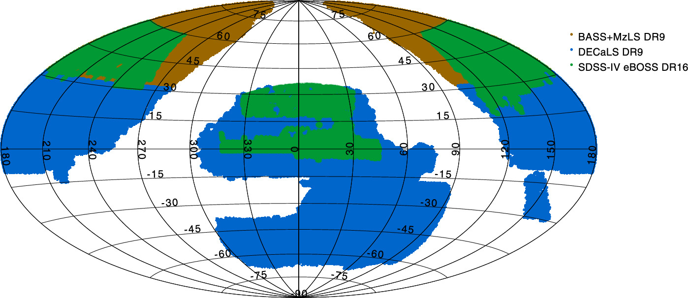
Figure 1. Spatial coverage of the two samples used in this work. The photometric sample is the Legacy Surveys DR9, where the DECaLS part is shown in the blue color and the BASS+MzLS part is represented by the dark orange color. The spectroscopic sample is SDSS-IV eBOSS DR16, with quasars shown in the green color.
Download figure:
Standard image High-resolution image2.3. Completeness and Designs
As in Xu et al. (2022b), we employ the z-band 10σ point-source depth to assess the mass completeness of photometric objects. This analysis is conducted within the matched footprint of the Legacy Surveys and the eBOSS quasar sample. As presented in Figure 2, 90% of the regions covered by the Legacy Surveys are deeper than 22.34 in z band. Therefore, we take z = 22.34 as the galaxy depth for the Legacy Surveys.
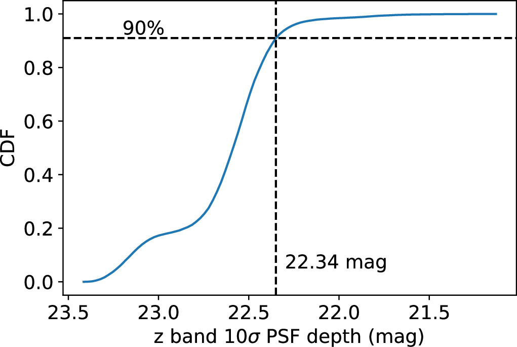
Figure 2. Cumulative distribution function of the survey area to the z-band 10σ point-source depth in the Legacy Surveys matched with the eBOSS quasar footprint.
Download figure:
Standard image High-resolution imageWe calculate the galaxy physical properties using the SED code CIGALE (Boquien et al. 2019) with grz-band fluxes. We adopt the stellar spectral library provided by Bruzual & Charlot (2003) to build up stellar population synthesis models. The initial stellar mass function in Chabrier (2003) is assumed. We take Z/Z⊙ = 0.4, 1.0, and 2.5 as three different metallicities in our model. A delayed star formation history  is taken, with the timescale τ varying from 107 to 1.258 × 10¹⁰ yr with an equal logarithm space of 0.1 dex. We apply the starburst reddening law of Calzetti et al. (2000) to consider the dust attenuation, in which the color excess E(B − V) changes from 0 to 0.5.
Following Xu et al. (2022b), we select the deepest 50 deg2 regions in the Legacy Surveys, comprising 738 bricks, where the z-band 10σ point-source depth exceeds 23.37, to study the stellar mass completeness C95(M*), with the photometric redshift (zp) calculated by Zhou et al. (2021). C95(M*) is defined such that 95% of the galaxies are brighter than C95(M*) in z band for a given stellar mass M*. In Figure 3, we show the stellar mass z-band magnitude distribution of the deep photometric sample at redshift 0.8 < zp < 1.0. We mark C95(M*) with the red line in Figure 3, from which the complete stellar mass is 1010.80 M⊙ at redshift 0.8 < zs < 1.0 for the z-band depth of 22.34. Hence, we use the stellar mass of photometric objects at the interval of [1010.80, 1011.80] M⊙ at redshift 0.8 < zs < 1.0 separated by four equal redshift bins. Furthermore, to constrain the SHMR at lower masses, we incorporate the incomplete stellar mass bins within the range of [1010.00, 1010.80] M⊙ through appropriate modeling, as illustrated later.
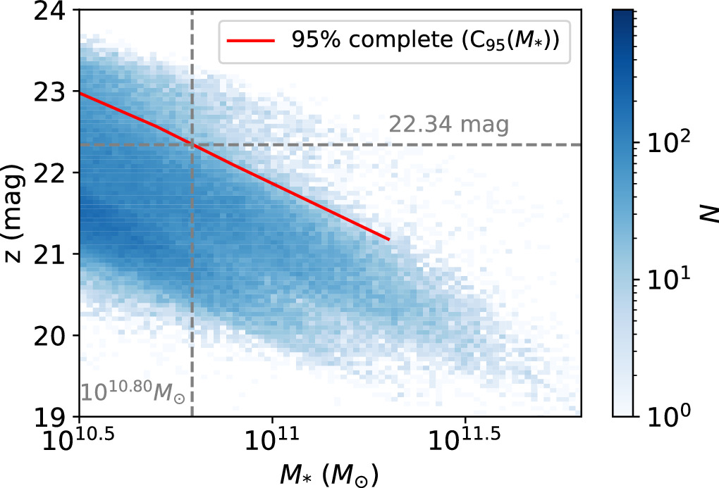
Figure 3. The distribution of stellar mass vs. z-band magnitude for DECaLS DR9 galaxies with photo-z between 0.8 and 1.0. The red line represents the faint z-band magnitude limit such that 95% of galaxies at each stellar mass are brighter than the limit. The horizontal gray dashed line shows the survey depth in the z band determined in Figure 2. The vertical gray dashed line is the completeness limit at stellar mass 1010.8 M⊙ for the photometric galaxies at the redshift of our interest.
Download figure:
Standard image High-resolution image2.4. Measurements
We follow the approach in Xu et al. (2022a) to average the result at different sky regions and redshift bins with proper weights to acquire the final  .
.
For representational simplicity, let  . Supposing
  is calculated for Nr
redshift bins and Ns
sky regions, we further divide each region into Nsub subregions for error estimation. In our specific scenario, Nr
is set to 4, corresponding to the redshift bins [0.80, 0.85], [0.85, 0.90], [0.90, 0.95], and [0.95, 1.00]. Additionally, Ns
is defined as 3, representing BASS+MzLS NGC, DECaLS SGC, and DECaLS NGC, while Nsub is established as 10. According to Equation (1),
is calculated for Nr
redshift bins and Ns
sky regions, we further divide each region into Nsub subregions for error estimation. In our specific scenario, Nr
is set to 4, corresponding to the redshift bins [0.80, 0.85], [0.85, 0.90], [0.90, 0.95], and [0.95, 1.00]. Additionally, Ns
is defined as 3, representing BASS+MzLS NGC, DECaLS SGC, and DECaLS NGC, while Nsub is established as 10. According to Equation (1),  can be measured in the ith redshift bin, jth sky region, and kth subsample through the Landy–Szalay estimator (Landy & Szalay 1993). First, we average the measurements at different sky regions using the region area ws,j as a weighting factor to take the sky area difference into account:

Second, we obtain the mean values and the error vector σi of the mean values for each redshift bin from Nsub subsamples:

Finally, the results from different redshift bins are averaged according to the error vector σi
. Let  ,
,
We measure  and the autocorrelation wp of quasars in the radial range of 0.1 h−1 Mpc < rp < 15 h−1 Mpc. These scales are sufficiently broad to capture the distributions of both centrals and satellites. The measurements of
  are depicted as data points with error bars in Figure 4. The error bars represent the vector σ. These measurements are overall good across all stellar mass bins within the entire radial range, except for the highest-stellar-mass bin [1011.6, 1011.8] M⊙. Additionally, the autocorrelation wp of quasars, with the weights assigned in the same way as in Hou et al. (2021), is presented in Figure 5 to enhance the precision in constraining the mean host halo mass of quasars.
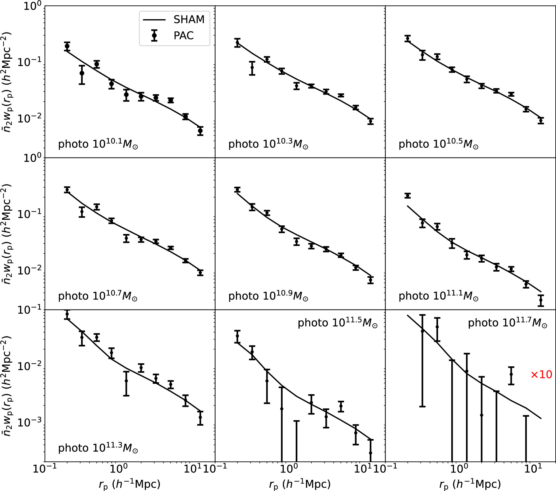
Figure 4. The measurements (data points with error bars) and the model fitting (lines) of the excess projected density  of galaxies around eBOSS quasars. The stellar mass of galaxies ranges from 1010.0
M⊙ to 1011.8
M⊙, as the median mass indicated in each panel. The results for the highest-stellar-mass bin (1011.7
M⊙) are multiplied by 10.
of galaxies around eBOSS quasars. The stellar mass of galaxies ranges from 1010.0
M⊙ to 1011.8
M⊙, as the median mass indicated in each panel. The results for the highest-stellar-mass bin (1011.7
M⊙) are multiplied by 10.
Download figure:
Standard image High-resolution image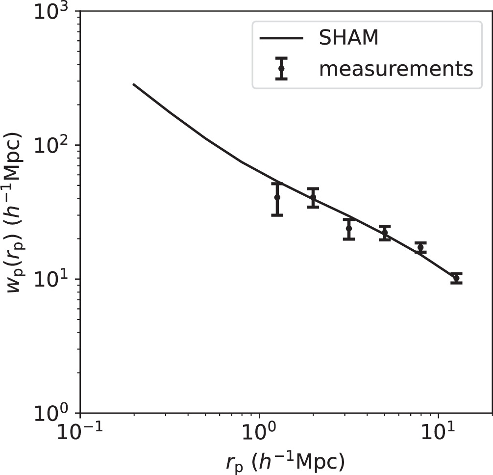
Figure 5. The measurements (data points with error bars) and the model fitting (line) of the projected autocorrelation wp of quasars.
Download figure:
Standard image High-resolution image3. Simulation and Results
In this section, we outline the N-body simulation and the SHAM method employed in this study for modeling the measurements. We present the best-fit results for the SHMR within the redshift range of 0.8 < zs < 1.0 and explore the quasar–halo connection. Additionally, we highlight the high satellite fraction of quasars from our findings and assess the assumptions underlying the model.
3.1. N-body Simulation
We employ the CosmicGrowth simulation suite (Jing 2019), a grid of high-resolution N-body simulations utilizing the computationally efficient adaptive parallel P3M method (Jing & Suto 2002; Xu & Jing 2021). We utilize the ΛCDM simulation with the following cosmological parameters: Ωm,0 = 0.268, ΩΛ,0 = 0.732, h = 0.71, ns = 0.968, and σ8 = 0.83. This simulation comprises 30723 dark matter particles within a 600 h−1 Mpc box, with a softening length of η = 0.01 h−1 Mpc. Groups are characterized with the friends-of-friends algorithm (Davis et al. 1985), employing a linking length of 0.2 times the mean particle separation. The halos are then processed with HBT+ (Han et al. 2012, 2018), to identify subhalos and trace their evolution histories. Merger timescales of the subhalos with fewer than 20 particles are estimated using the fitting formula in Jiang et al. (2008). Subhalos that have already merged into central subhalos are disregarded. The adopted simulation has a mass resolution of mp = 5.54 × 10⁸ h−1 M⊙, which proves to be sufficiently fine for our study. We utilize snapshot 76 at a redshift of approximately 0.92 to align with the observations.
3.2. SHAM
To associate galaxies with (sub)halos in the N-body simulation, we implement the SHAM method. We utilize the widely used five-parameter formula for the SHMR, a double power law with a constant scatter (Wang & Jing 2010; Yang et al. 2012; Moster et al. 2013; Xu et al. 2023):
Here, Macc is defined as the virial mass Mvir of the (sub)halo when it was last to become a central dominant object, where Mvir is defined through the fitting formula in Bryan & Norman (1998). The scatter in  at a given Macc is assumed to follow a Gaussian distribution with a width of σ. The same set of parameters is applied for both centrals and satellites (Wang & Jing 2010; Behroozi et al. 2019; Xu et al. 2023).
In addition to the standard SHAM parameters described above, given the inclusion of measurements from incomplete stellar mass bins, we introduce four additional parameters k1, k2, k3, and k4 to account for the incompleteness of the four stellar mass bins. The modeled results from the simulation are obtained by multiplying the  from the entire sample by the incompleteness, under the assumption that the incompleteness only affects the amplitude of the observed
  .
.
To associate quasars with (sub)halos, we assume that the probability that a (sub)halo hosts a quasar follows a Gaussian distribution of logarithmic halo mass ![${\mathrm{log}}_{10}[{M}_{\mathrm{acc}}/({h}^{-1}\,{M}_{\odot })]$](https://content.cld.iop.org/journals/0004-637X/967/1/17/revision1/apjad3b96ieqn30.gif) , with a mean value μ and a dispersion σq. We use the same μ and σq for both halos and subhalos, Further, we introduce an additional parameter B to adjust the overall probability for a subhalo to host a quasar relative to a halo at the same mass. This ensures that the subhalos have B times the probability of hosting a quasar relative to a halo of the same mass. Under the above schedule, the satellite fraction fs of quasars is defined as:
, with a mean value μ and a dispersion σq. We use the same μ and σq for both halos and subhalos, Further, we introduce an additional parameter B to adjust the overall probability for a subhalo to host a quasar relative to a halo at the same mass. This ensures that the subhalos have B times the probability of hosting a quasar relative to a halo of the same mass. Under the above schedule, the satellite fraction fs of quasars is defined as:

where Nsate and Ncen represent the numbers of subhalos and halos selected based on the same Gaussian distribution.
After assigning galaxies and quasars to (sub)halos, we compute the correlation functions using Corrfunc (Sinha & Garrison 2020) in the simulation. To compare with the measurements in observations, we define the χ2 as:
Here, Nm and Nr denote the numbers of stellar mass bins and of radial bins, respectively. We explore the parameter space using the Markov Chain Monte Carlo (MCMC) sampler emcee (Foreman-Mackey et al. 2013), employing maximum likelihood analyses for the three sets of parameters {M0, α, β, k, σ}, {k1, k2, k3, k4}, and {μ, σq, B}.
3.3. SHMR and Quasar–Halo Connection
The best-fit results and errors for the parameters are presented in the first row of Table 1. Additionally, the joint posterior distributions of the parameters are illustrated in Figure A1 using corner (Foreman-Mackey 2016). The best-fit  and wp results from the model are shown in Figures 4 and 5 with solid lines. The fits are generally good for all stellar mass bins, both on the small and large scales.
Table 1. The Best-fit Parameter Results and Errors for the SHMR, Incompleteness, and Quasar–Halo Connection, Assuming a Gaussian Distribution for the Quasar Probability

| α | β |

| σ | μ | σq | k1 | k2 | k3 | k4 | B |
|---|---|---|---|---|---|---|---|---|---|---|---|

|

|

|

|

|

|

|

|

|

|

|

|

|

|

|

|

|

| 0.50 (set) |

|

|

|

|

|
Note. The first row displays the fiducial results with all parameters free, while the second row presents the results for the remaining parameters after setting σq to 0.5. M0 is in units of h−1 M⊙ and k is in M⊙.
Download table as: ASCIITypeset image
For quasars, we find that μ, σq, and B are  ,
,  , and
, and  , respectively. The results indicate a very high satellite fraction of quasars, with
  . B is equal to 1 within the 1σ error, implying that subhalos have nearly the same chance of hosting quasars as the halos and that quasar activity is not affected by the larger halo environment. After determining the host halo masses for subhalos and adjusting the number density of quasars to match the observed value of approximately 1.29 × 10⁻⁵
h3 Mpc−3, we illustrate the HOD of our quasar sample in Figure 6. We obtain median host halo masses for central and satellite quasars of
. B is equal to 1 within the 1σ error, implying that subhalos have nearly the same chance of hosting quasars as the halos and that quasar activity is not affected by the larger halo environment. After determining the host halo masses for subhalos and adjusting the number density of quasars to match the observed value of approximately 1.29 × 10⁻⁵
h3 Mpc−3, we illustrate the HOD of our quasar sample in Figure 6. We obtain median host halo masses for central and satellite quasars of ![${\mathrm{log}}_{10}[{M}_{{\rm{h}},\mathrm{cen}}^{\mathrm{med}}/({h}^{-1}\,{M}_{\odot })]={12.05}_{-0.60}^{+0.60}$](https://content.cld.iop.org/journals/0004-637X/967/1/17/revision1/apjad3b96ieqn61.gif) and
and ![${\mathrm{log}}_{10}[{M}_{{\rm{h}},\mathrm{sat}}^{\mathrm{med}}/({h}^{-1}\,{M}_{\odot })]={12.90}_{-0.72}^{+0.68}$](https://content.cld.iop.org/journals/0004-637X/967/1/17/revision1/apjad3b96ieqn62.gif) . From the HOD, we observe that although the satellite fraction of quasars looks very high, each massive halo, on average, does not host more than one satellite quasar, due to the low total number density of quasars. To more effectively depict the mass distributions, we also present the host halo mass distributions for central and satellite quasars in Figure B1.
. From the HOD, we observe that although the satellite fraction of quasars looks very high, each massive halo, on average, does not host more than one satellite quasar, due to the low total number density of quasars. To more effectively depict the mass distributions, we also present the host halo mass distributions for central and satellite quasars in Figure B1.
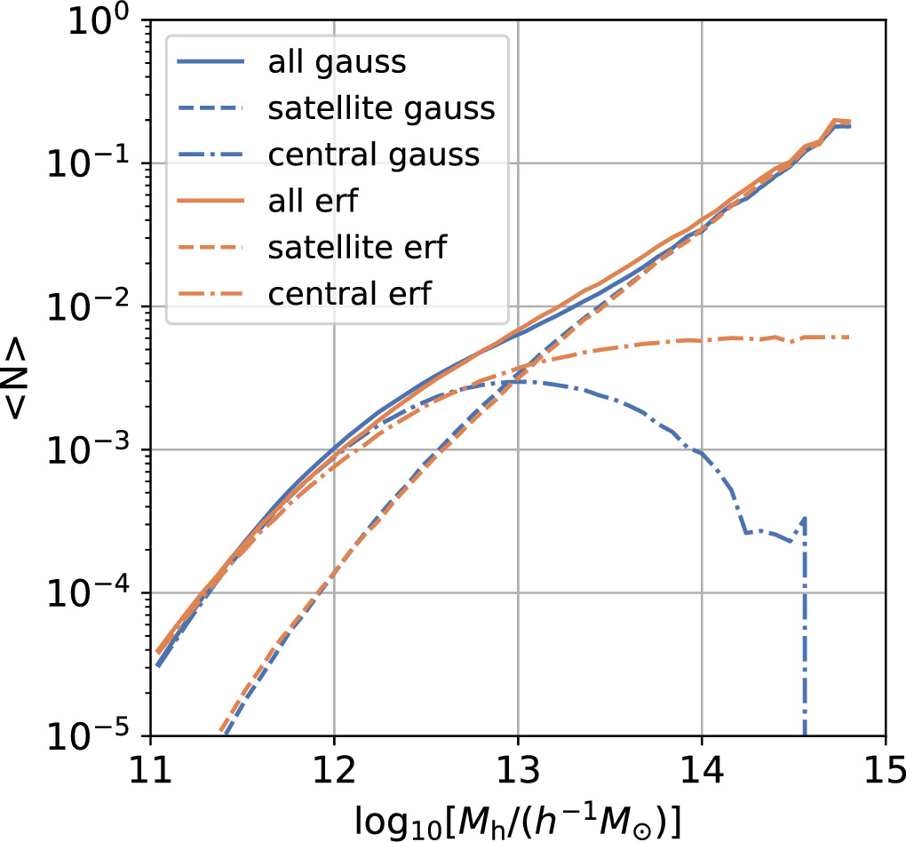
Figure 6. The mean HODs of quasars computed with the best-fit parameters. The results based on the Gaussian function for the quasar–halo relation are displayed in blue, with the parameters from the first row of Table 1. For comparison, the results based on the error function are shown in orange, with the parameters from Table 2. Central and satellite quasars are depicted by dotted and dotted–dashed lines, respectively.
Download figure:
Standard image High-resolution imageFor galaxies, we present the SHMR at 0.8 < zs < 1.0 in Figure 7, with ![${\mathrm{log}}_{10}[{M}_{0}/({h}^{-1}\,{M}_{\odot })]={11.83}_{-0.07}^{+0.06}$](https://content.cld.iop.org/journals/0004-637X/967/1/17/revision1/apjad3b96ieqn63.gif) ,
,  ,
,  ,
,  , and
, and  , extending the findings from Xu et al. (2023) to higher redshifts. Our results underscore the potential of leveraging quasars as high-redshift tracers for investigating galaxy formation. However, larger quasar samples and deeper photometric catalogs are required to more precisely constrain the low-mass end (e.g., β in SHMR) and to explore higher redshifts.
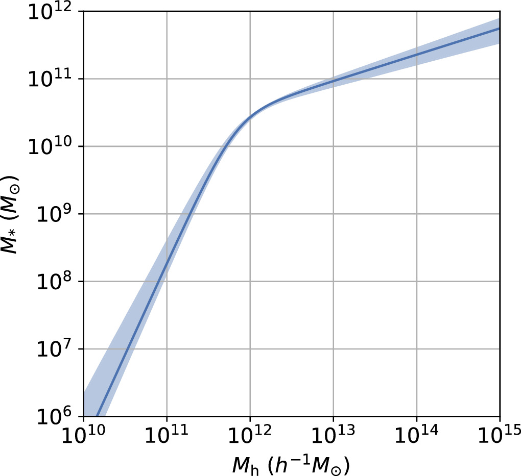
Figure 7. The SHMR at redshift 0.8 < zs < 1.0. The mean SHMR and 1σ errors are shown with blue line and shadow.
Download figure:
Standard image High-resolution imageMoreover, we determine the incompleteness of the photometric samples for the four lowest-stellar-mass bins, yielding  ,
,  ,
,  , and
, and  . These results highlight the capability of the PAC method to constrain the stellar mass incompleteness of photometric samples and utilize the incomplete sample to explore lower-mass regions.
3.4. Testing the Robustness of the Results
The satellite fraction of quasars in our results is  . This high satellite fraction suggests that subhalos have nearly the same probability (
 ) as halos of hosting quasars for the same host (infall) mass and that the large-scale environment has little effect on quasar activity. To verify the robustness of such a high satellite fraction of quasars, we conducted three tests, as follows. Since BASS is a bit shallower in the g and r bands than DECaLs, we measure
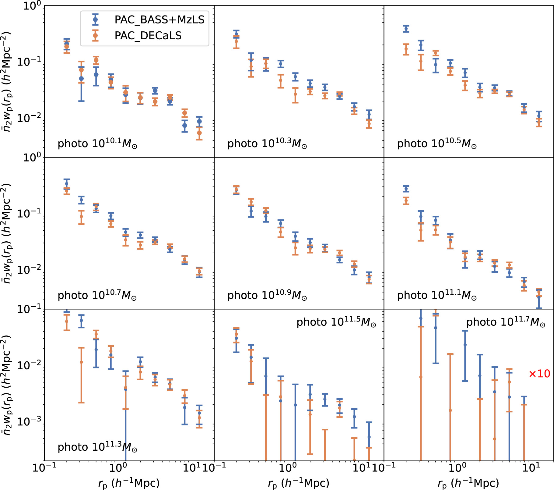
  in DECaLS and BASS, respectively, and a comparison of the results shows that the measurement is robust (Figure C1).
Initially, we observe a degeneracy between the parameters μ and σq in Figure A1. To investigate the impact of this degeneracy on the satellite fraction of quasars, we fix σq at 0.50, a value consistent with Richardson et al. (2012), and constrain the remaining parameters through MCMC analysis. The resulting best-fit parameters are presented in the second row of Table 1, and we find that a high satellite fraction is still necessary to align with the observations and that all parameters remain consistent with the previous results within the 1σ interval. For better clarity, we depict the  results under these best-fit parameters for two stellar mass bins (1010.5
M⊙ and 1010.9
M⊙) in Figure 8 using solid blue lines. We find that the measurements can also be well fitted by this model. This test confirms that the satellite fraction of quasars remains unaffected by the degeneracy between μ and σq.
results under these best-fit parameters for two stellar mass bins (1010.5
M⊙ and 1010.9
M⊙) in Figure 8 using solid blue lines. We find that the measurements can also be well fitted by this model. This test confirms that the satellite fraction of quasars remains unaffected by the degeneracy between μ and σq.
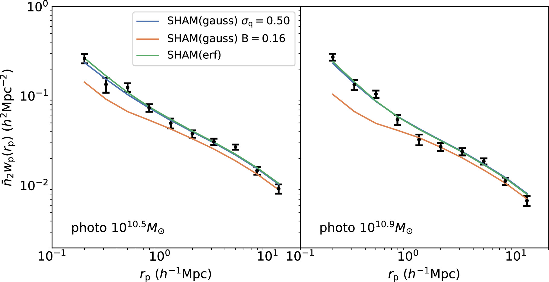
Figure 8. The  measurements in two stellar mass bins, 1010.5
M⊙ and 1010.9
M⊙. The dots with error bars represent the observational measurements. The orange solid lines depict the best-fit results with fsate set to 0.05 (equivalently B = 0.16), while keeping other parameters the same as in the first row of Table 1. The blue solid lines show the best-fit results with σq set to 0.50. The green solid lines represent the best-fit results assuming a probability of a (sub)halo hosting a quasar modeled by an error function.
measurements in two stellar mass bins, 1010.5
M⊙ and 1010.9
M⊙. The dots with error bars represent the observational measurements. The orange solid lines depict the best-fit results with fsate set to 0.05 (equivalently B = 0.16), while keeping other parameters the same as in the first row of Table 1. The blue solid lines show the best-fit results with σq set to 0.50. The green solid lines represent the best-fit results assuming a probability of a (sub)halo hosting a quasar modeled by an error function.
Download figure:
Standard image High-resolution imageSecond, to examine whether a low satellite fraction of quasars, as suggested by some previous studies (Richardson et al. 2012; Shen et al. 2013), is consistent with our measurements, we set the B parameter to be 0.16, corresponding to fsate = 0.05 according to Equation (8), while keeping the remaining parameters unchanged. The simulation results in two stellar mass bins (1010.5
M⊙ and 1010.9
M⊙) are presented in Figure 8 with solid orange lines. In this case, we observe that the model fails to match the steep increase of  at small scales (rp < 1 h−1 Mpc), suggesting that a higher satellite fraction is required to reproduce the observation.
Third, considering our assumption of a Gaussian format for the quasar probability in our modeling, we aim to verify whether this assumption affects the satellite fraction of quasars. Therefore, we replace the Gaussian format with the error function format for both the central and satellite quasars shown, as follows:
where P(Mh) is the probability of a halo becoming a quasar.  and
and  are the characteristic mass scale and transition width of a softened step function. The best-fit parameters are presented in Table 2, where we still find a high satellite fraction of quasars, indicated by the parameter
  with
with  . For a clearer illustration, simulation results in two stellar mass bins (1010.5
M⊙ and 1010.9
M⊙) are shown in Figure 8 with solid green lines. We observe that the measurements can also be well fitted by this model. To compare the difference between the Gaussian format and the error function, we show the HOD from the error function model in Figure 6. We observe that the HODs for satellites are nearly identical for these two models. Although some discrepancy is found for centrals with Mh > 1013.0
M⊙, this does not significantly impact fsate, due to the low number densities of these massive halos. This test confirms that our results are not sensitive to the assumptions in the quasar–halo connection.
. For a clearer illustration, simulation results in two stellar mass bins (1010.5
M⊙ and 1010.9
M⊙) are shown in Figure 8 with solid green lines. We observe that the measurements can also be well fitted by this model. To compare the difference between the Gaussian format and the error function, we show the HOD from the error function model in Figure 6. We observe that the HODs for satellites are nearly identical for these two models. Although some discrepancy is found for centrals with Mh > 1013.0
M⊙, this does not significantly impact fsate, due to the low number densities of these massive halos. This test confirms that our results are not sensitive to the assumptions in the quasar–halo connection.
Table 2. The Best-fit Parameter Results and Errors for the SHMR, Incompleteness, and Quasar–Halo Connection, Assuming an Error Function for the Quasar Probability

| α | β |

| σ |

|

| k1 | k2 | k3 | k4 | B |
|---|---|---|---|---|---|---|---|---|---|---|---|

|

|

|

|

|

|

|

|

|

|

|

|
Note.
M0 and  are in units of h−1
M⊙ and k is in M⊙.
are in units of h−1
M⊙ and k is in M⊙.
Download table as: ASCIITypeset image
Our higher satellite fraction of quasars than that determined by Shen et al. (2013) may come from two sources. One is the measurements of the cross-correlation between galaxies and quasars. In this paper, we have used galaxies with stellar mass larger than 1010.0
M⊙, compared with the LRGs used by Shen et al. (2013). While we find the slopes of the cross-correlation functions within rp = 1 h−1 Mpc are consistent for massive galaxies (i.e., >1011.2
M⊙) between the two works, our measurement for less massive galaxies also requires more satellite quasars around small central galaxies (see the left panel of Figure 8). The other source is different assumptions for the modeling. We use the abundance-matching method, while Shen et al. (2013) used the HOD method. We note that the satellite fraction is quite sensitive to the HOD forms used for the central quasars in Shen et al. (2013). It changes from  when the error function form is used to
  when the lognormal form is used instead. Furthermore, they require satellite quasars to exist only in halos with Mh > 1013.0
h−1
M⊙ (see their Figure 14). In comparison, we allow many more small halos with Mh < 1013.0
h−1
M⊙ (Figure B1) to host satellite quasars, which are required to reproduce the cross-correlation between quasars and galaxies with stellar mass less than 1011.0
M⊙ (e.g., the left panel of Figure 8). Therefore, our higher satellite fraction mainly comes from those satellite quasars in halos with Mh < 1013.0
h−1
M⊙ that were not probed by Shen et al. (2013). Because central halos as small as Mh > 1011.5
h−1
M⊙ can host quasars in the both works (see their Figure 14 and our Figure 6), it is more reasonable that halos with Mh < 1013.0
h−1
M⊙ can host satellite quasars, as there are subhalos that are massive enough.
when the lognormal form is used instead. Furthermore, they require satellite quasars to exist only in halos with Mh > 1013.0
h−1
M⊙ (see their Figure 14). In comparison, we allow many more small halos with Mh < 1013.0
h−1
M⊙ (Figure B1) to host satellite quasars, which are required to reproduce the cross-correlation between quasars and galaxies with stellar mass less than 1011.0
M⊙ (e.g., the left panel of Figure 8). Therefore, our higher satellite fraction mainly comes from those satellite quasars in halos with Mh < 1013.0
h−1
M⊙ that were not probed by Shen et al. (2013). Because central halos as small as Mh > 1011.5
h−1
M⊙ can host quasars in the both works (see their Figure 14 and our Figure 6), it is more reasonable that halos with Mh < 1013.0
h−1
M⊙ can host satellite quasars, as there are subhalos that are massive enough.
4. Conclusions
In this paper, we utilize a spectroscopic quasar sample from SDSS-IV eBOSS DR16 and a photometric galaxy sample from the Legacy Surveys. We employ the PAC method to measure  between quasars and galaxies, in conjunction with the quasar autocorrelation wp, at redshift 0.8 < zs < 1.0. Leveraging the advantages of PAC, we obtain reliable quasar clustering down to 0.1 h−1 Mpc. We model the measurements in N-body simulations using the SHAM approach and assume a Gaussian probability for a (sub)halo to host a quasar. We constrain the SHMR of galaxies and the quasar–halo connection. We verify the assumptions and confirm that a high satellite fraction of quasars is required to reproduce the observations. The main results are listed as follows:
- 1.Under the assumption that the probability of a halo becoming a quasar follows a Gaussian distribution of logarithmic halo mass, we find that the median host halo masses for central and satellite quasars are and at redshift 0.8 < zs < 1.0 and a high satellite fraction of quasars of . This high satellite fraction of quasars indicates that subhalos have nearly the same probability of hosting quasars as halos for the same host (infall) mass and that the large-scale environment has little effect on the quasar activity.
- 2.We constrain the SHMR of galaxies at redshift 0.8 < zs < 1.0, which can be described by a double power law with, , , , and . These results underscore the potential of leveraging quasars as high-redshift tracers for investigating galaxy formation.
![${\mathrm{log}}_{10}[{M}_{{\rm{h}}}/({h}^{-1}\,{M}_{\odot })]$](https://content.cld.iop.org/journals/0004-637X/967/1/17/revision1/apjad3b96ieqn102.gif)
![${\mathrm{log}}_{10}[{M}_{{\rm{h}},\mathrm{cen}}^{\mathrm{med}}/({h}^{-1}\,{M}_{\odot })]={12.05}_{-0.60}^{+0.60}$](https://content.cld.iop.org/journals/0004-637X/967/1/17/revision1/apjad3b96ieqn103.gif)
![${\mathrm{log}}_{10}[{M}_{{\rm{h}},\mathrm{sat}}^{\mathrm{med}}/({h}^{-1}\,{M}_{\odot })]={12.90}_{-0.72}^{+0.68}$](https://content.cld.iop.org/journals/0004-637X/967/1/17/revision1/apjad3b96ieqn104.gif)

![${\mathrm{log}}_{10}[{M}_{0}/({h}^{-1}\,{M}_{\odot })]={11.83}_{-0.07}^{+0.06}$](https://content.cld.iop.org/journals/0004-637X/967/1/17/revision1/apjad3b96ieqn106.gif)


With the forthcoming data from DESI (DESI Collaboration et al. 2023; Adame et al. 2024), we anticipate gaining a better understanding of quasar clustering, given the larger number of surveyed quasars compared to SDSS-IV. Additionally, with the quasar–halo connection determined by our SHAM method, we can generate quasar mocks for DESI. With future large and deep photometric surveys like the Legacy Survey of Space and Time (Ivezić et al. 2019) and Euclid (Laureijs et al. 2011), we can gather much more quasar clustering information with smaller stellar mass bins.
Acknowledgments
The work is supported by the NSFC (12133006, 11890691), grant No. CMS-CSST-2021-A03, and 111 project No. B20019. We gratefully acknowledge the support of the Key Laboratory for Particle Physics, Astrophysics and Cosmology, Ministry of Education. This work made use of the Gravity Supercomputer at the Department of Astronomy, Shanghai Jiao Tong University.
Funding for the Sloan Digital Sky Survey IV has been provided by the Alfred P. Sloan Foundation, the U.S. Department of Energy Office of Science, and the Participating Institutions. SDSS-IV acknowledges support and resources from the Center for High-Performance Computing at the University of Utah. The SDSS website is www.sdss.org.
SDSS-IV is managed by the Astrophysical Research Consortium for the Participating Institutions of the SDSS Collaboration, including the Brazilian Participation Group, the Carnegie Institution for Science, Carnegie Mellon University, the Chilean Participation Group, the French Participation Group, Harvard–Smithsonian Center for Astrophysics, Instituto de Astrofísica de Canarias, The Johns Hopkins University, Kavli Institute for the Physics and Mathematics of the Universe (IPMU)/University of Tokyo, Korean Participation Group, Lawrence Berkeley National Laboratory, Leibniz Institut für Astrophysik Potsdam (AIP), Max-Planck-Institut für Astronomie (MPIA Heidelberg), Max-Planck-Institut für Astrophysik (MPA Garching), Max-Planck-Institut für Extraterrestrische Physik (MPE), National Astronomical Observatories of China, New Mexico State University, New York University, University of Notre Dame, Observatário Nacional/MCTI, The Ohio State University, Pennsylvania State University, Shanghai Astronomical Observatory, United Kingdom Participation Group, Universidad Nacional Autónoma de México, University of Arizona, University of Colorado Boulder, University of Oxford, University of Portsmouth, University of Utah, University of Virginia, University of Washington, University of Wisconsin, Vanderbilt University, and Yale University.
The Legacy Surveys consist of three individual and complementary projects: the Dark Energy Camera Legacy Survey (DECaLS; Proposal ID #2014B-0404; PIs: David Schlegel and Arjun Dey), the Beijing–Arizona Sky Survey (BASS; NOAO Prop. ID #2015A-0801; PIs: Zhou Xu and Xiaohui Fan), and the Mayall z-band Legacy Survey (MzLS; Prop. ID #2016A-0453; PI: Arjun Dey). DECaLS, BASS, and MzLS together include data obtained, respectively, at the Blanco telescope, Cerro Tololo Inter-American Observatory, NSF's NOIRLab; the Bok telescope, Steward Observatory, University of Arizona; and the Mayall telescope, Kitt Peak National Observatory, NOIRLab. The Legacy Surveys project is honored to be permitted to conduct astronomical research on Iolkam Du'ag (Kitt Peak), a mountain with particular significance to the Tohono O'odham Nation.
Appendix A: Posterior Distributions of the Parameters
We present the posterior probability density functions of the 12 parameters in our fiducial model in this section, as shown in Figure A1.
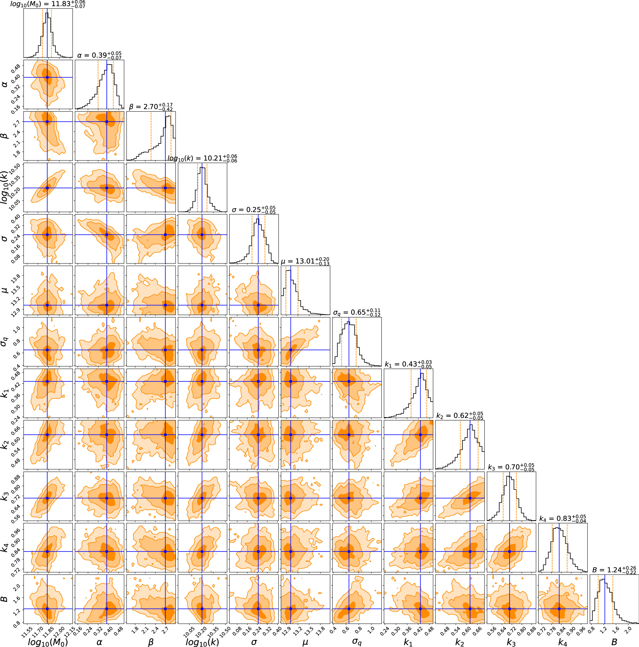
Figure A1. The posterior distributions of the 12 parameters in our model obtained through MCMC. The vertical green line indicates the median value of each parameter, and the dashed blue lines denote the 16th and 84th percentiles after marginalizing over the parameters.
Download figure:
Standard image High-resolution imageAppendix B: Host Halo Mass Distributions of Quasars
We present the mass distributions of the host halos of central and satellite quasars in Figure B1.
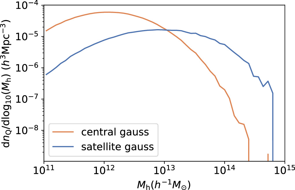
Figure B1. The number density distribution of the host halos of central and satellite quasars. The central and satellite quasars are marked with orange and blue solid lines, respectively.
Download figure:
Standard image High-resolution imageAppendix C: Comparison of Measurements

We compare the  measurements with the DR9 catalogs from DECaLS and from BASS+MzLS that are shown in Figure C1.
Figure C1. The measurement of  . Measurements with the DR9 catalog from DECaLS are shown in blue colors and measurements with the DR9 catalogs from BASS and MzLS are shown in orange colors.
Download figure:
Standard image High-resolution image
Footnotes
- 5
Throughout the paper, we use zs for spectroscopic redshift and z for the z-band magnitude.
- 6
- 7
- 8