


Abstract
Large amplitude Alfvénic fluctuations, sometimes leading to localized inversions of the magnetic field, called switchbacks, are a common but poorly understood phenomenon in the solar wind. In particular, their origin(s), evolution, and stability within solar wind conditions are yet to be fully understood. Simulations modeling switchbacks have previously studied their stability in 2D. Here, we investigate the decay process of Alfvén wave packets via MHD simulations in 3D by characterizing the effects of system size, aspect ratio, and propagation angle on the decay rate. We show that the initial wave packet is unstable to parametric instabilities that develop compressible and Alfvénic secondary modes in the plane of, and transverse to, the initial wave packet propagation direction. The growth of transverse modes, absent in 2D simulations, increases the decay rate of the wave packet. We finally discuss the implications of our results for lifetime estimates of switchbacks and wave energy conversion in the solar wind.
Export citation and abstract BibTeX RIS

Original content from this work may be used under the terms of the Creative Commons Attribution 4.0 licence. Any further distribution of this work must maintain attribution to the author(s) and the title of the work, journal citation and DOI.
1. Introduction
In the model of the solar wind introduced by Eugene Parker in 1958, the solar wind would blow outward smoothly from the Sun, and the magnetic field lines carried by it would extend out into the solar system, forming a spiral known as the Parker spiral (Parker 1958). However, since the first in situ measurements (Belcher & Davis 1971), it has become clear that the solar wind is a much more complex system than what was predicted by Parker's laminar model. The solar wind is, in fact, a turbulent medium permeated by large-amplitude fluctuations, mostly in the velocity and magnetic fields. Furthermore, some solar wind streams, those referred to as Alfvénic streams, are typically faster and hotter than what traditional theories predict (Vasquez et al. 2007; Hellinger et al. 2011, 2013). Understanding turbulence and fluctuations is therefore critical to understanding the acceleration of the wind and the origin of plasma heating (Hellinger et al. 2013; Cranmer et al. 2015; Viall & Borovsky 2020).
Solar wind fluctuations sometimes lead to kinks in the magnetic field, often called switchbacks because the magnetic field can reverse direction even up to 180°, although they are also known by other names such as kinks, jets, and spikes (Horbury et al. 2020). The Parker Solar Probe mission has confirmed that switchbacks are ubiquitous and exist at various time and spatial scales within the solar wind (Dudok de Wit et al. 2020; Bale et al. 2021; Shi et al. 2022), adding to previous observations of switchbacks at larger radial distances from the Sun, from 0.3 ≲ R ≲ 1 au (Horbury et al. 2018) to R ≳ 1 au (Balogh et al. 1999; Gosling et al. 2009; Matteini et al. 2014). With the new data from the Parker Solar Probe, a debate about the origin of switchbacks is burning as hot as the Sun. Recent evidence from the Parker Solar Probe points to magnetic reconnection, and places switchback formation in the coronal region (Zank et al. 2020; Drake et al. 2021; Bale et al. 2023). The difficulty then is explaining how switchbacks survive as far out as they have been observed. Other investigations suggest that switchbacks form from Alfvénic turbulence within the solar wind itself, due to effects such as expansion (Squire et al. 2020; Shoda et al. 2021; Johnston et al. 2022) or velocity shears (Landi et al. 2006; Toth et al. 2023). It will will require some combination of these theories in order to correctly mesh data with simulated models. Critical to the discussion is, once formed, how long switchbacks can survive in the solar wind, and what role, if any, they play in the evolution of solar wind turbulence and heating.
Switchbacks are large-amplitude Alfvénic fluctuations with nearly constant magnetic field strength. Thus, understanding how they form, propagate, and eventually decay requires understanding Alfvén waves in general. It is well known that Alfvén waves of large amplitude are subject to parametric instability, which causes the wave to decay into forward- and backward-propagating daughter waves. Such a process has been studied theoretically and numerically through a wide range of conditions, and in both fluid and kinetic descriptions of the plasma (Derby 1978; Goldstein 1978; Vinas & Goldstein 1991; Malara & Velli 1996; Matteini et al. 2010; Del Zanna et al. 2015; Primavera et al. 2019). However, most of the past investigations have focused on the decay of Alfvén waves or broadband spectra that fill space homogeneously. Recently, Tenerani et al. (2020) investigated the dynamics of a localized two-dimensional Alfvén wave packet in a homogeneous plasma by two-dimensional magnetohydrodynamic (MHD) simulations. They showed that a localized large-amplitude kink of the magnetic field is significantly more stable than a volume-filling wave spectrum and can propagate up to a few hundred Alfvén times before decaying by parametric instability.
In this paper, we extend the work of Tenerani et al. (2020) through three-dimensional MHD simulations of an Alfvén wave packet similar to a switchback. We find that additional coupling with fast and slow modes develops in the direction transverse to the plane of the kink and contributes to its decay. We describe the modes formed from the instability and their growth rates with different geometries of the wave packet, and finally discuss implications for lifetime estimates of switchbacks and wave energy conversion in the solar wind.
2. Model and Numerical Setup
We consider a kinked Alfvén wave packet that is initially characterized by a constant total magnetic field strength B. One of the distinctive characteristics of Alfvénic fluctuations in the solar wind is that they display a nearly constant total magnetic field strength. Such an observed property plays a crucial role in the stability of highly kinked Alfvénic wave packets (Tenerani et al. 2020). Furthermore, it ensures that fluctuations with correlated velocity and magnetic fields like Alfvén waves provide an exact solution to the compressible, nonlinear MHD system. Here, we use a reduced two-dimensional model (Landi et al. 2005; Tenerani et al. 2020) to build a kinked wave packet. To this end, we take a 2D scalar potential ψ(x, z) and define the magnetic field as

where  is the background, guiding magnetic field. To obtain By
, we impose the condition of constant magnetic field strength,
is the background, guiding magnetic field. To obtain By
, we impose the condition of constant magnetic field strength,

The velocity fluctuation is then obtained by imposing the Alfvénic correlation  , where δ
B
corresponds to the fluctuating part of the magnetic field and ρ0 the initial uniform plasma density. We define the magnetic potential as follows:
, where δ
B
corresponds to the fluctuating part of the magnetic field and ρ0 the initial uniform plasma density. We define the magnetic potential as follows:

where

The magnetic field given by Equations (1)–(4) corresponds to a 2.5D kinked Alfvén wave packet (three-dimensional vectors depending on two spatial coordinates). The kink is in the x−z plane of a 3D box, invariant in the y-direction, and propagating along  at the Alfvén speed of
  .
.
Here, lengths are normalized to a reference length L, the magnetic field to B0, density to ρ0, speed to the corresponding Alfvén speed, and plasma pressure to magnetic pressure. In this work, we fix  and ∣x1 − x2∣ = ∣z1 − z2∣ = 2, while considering different aspect ratios lx
/lz
and amplitudes ψ0 of the wave packet. In particular, we choose lz
= 1, with lx
= 1.5 or lx
= 3, and ψ0 = 2 or ψ0 = 1.5. A summary of the parameters used can be found in Table 1. Figure 1 shows the profile of the magnetic field at the center of the box as a function of x (panel (a)) and as a function of z (panel (b)) for lx
/lz
= 1.5 and ψ0 = 2. Panel (c) shows a 3D plot of the magnetic field, with the background B0 = 1 removed to show the gradient scaling of the fluctuation.
and ∣x1 − x2∣ = ∣z1 − z2∣ = 2, while considering different aspect ratios lx
/lz
and amplitudes ψ0 of the wave packet. In particular, we choose lz
= 1, with lx
= 1.5 or lx
= 3, and ψ0 = 2 or ψ0 = 1.5. A summary of the parameters used can be found in Table 1. Figure 1 shows the profile of the magnetic field at the center of the box as a function of x (panel (a)) and as a function of z (panel (b)) for lx
/lz
= 1.5 and ψ0 = 2. Panel (c) shows a 3D plot of the magnetic field, with the background B0 = 1 removed to show the gradient scaling of the fluctuation.
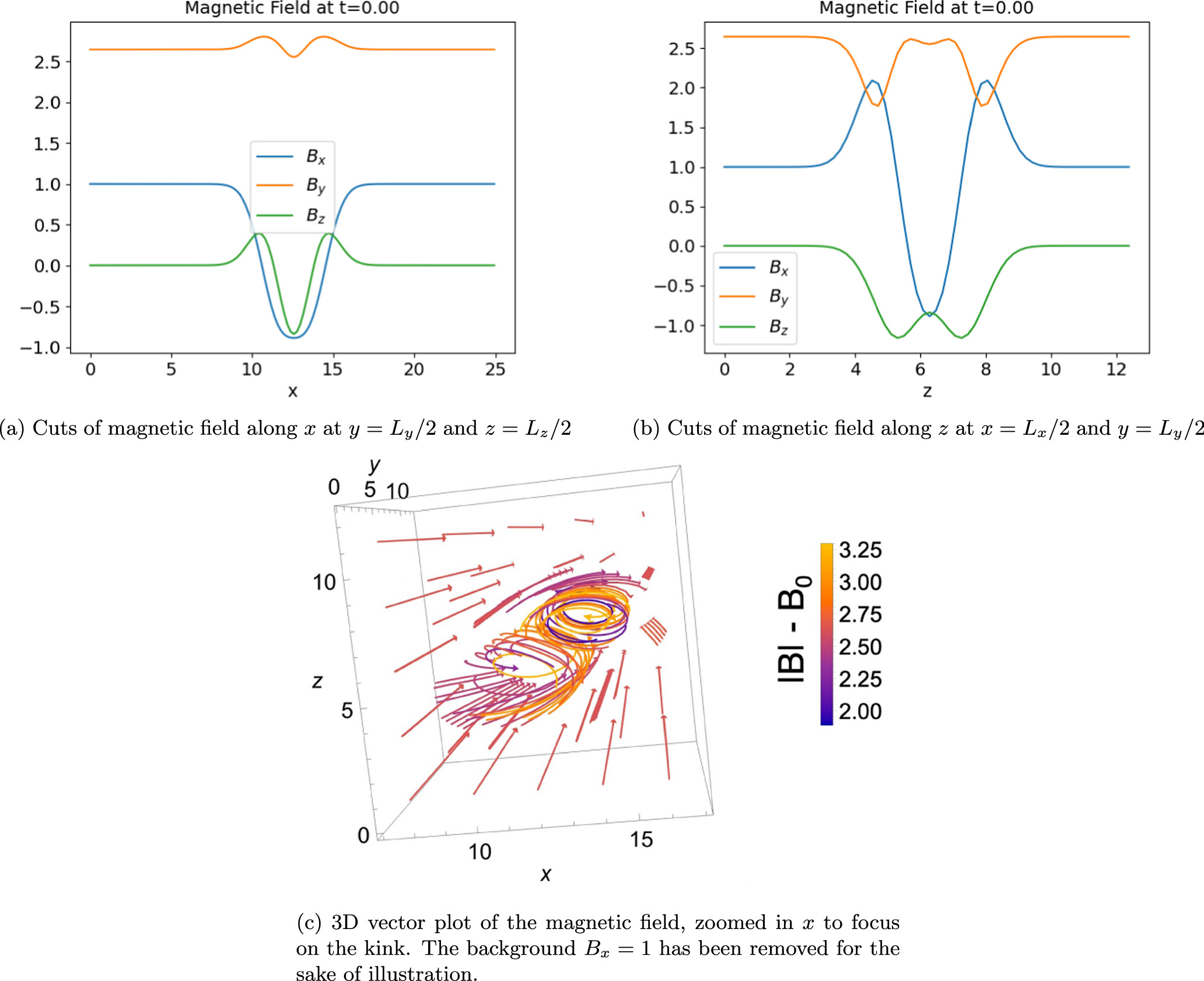
Figure 1. Initial profile of the magnetic field for box length Lx = 8π, aspect ratio lx /lz = 1.5, and amplitude ψ0 = 2. Note that the negative values in the x-components indicate the formation of a field reversal along the guiding field.
Download figure:
Standard image High-resolution imageTable 1. Summary of Our Simulations
| Run | Lx | lx /lz | θ | γ:ky (0) | γ:ky (1) | τ/ta |
|---|---|---|---|---|---|---|
| 0 | 8π | 1.5 | 69° | 0.017 ± 1 | 0.115 ± 3 | 230 |
| 4 | 16π | 1.5 | 69° | 0.017 ±2 | 0.037 ± 2 | 290 |
| 5 | 24π | 1.5 | 69° | 0.0105 ± 2 | 0.033 ± 1 | 360 |
| 6 | 32π | 1.5 | 69° | 0.0144 ± 4 | 0.0395 ± 1 | 480 |
| 7 | 64π | 1.5 | 69° | 0.0142 ± 2 | 0.0439 ± 7 | 415 |
| 8 | 72π | 1.5 | 69° | 0.0148 ± 3 | 0.0347 ± 9 | 455 |
| 9 | 16π | 3 | 69° | 0.0258 ± 9 | 0.0087 ± 1 | 230 |
| 10 | 4π | 1.5 | 35° | 0.0007 ± 0* | 0.0200 ± 2 | ⋯ |
Notes. Lx is the box length along the wave packet propagation direction, lx /lz is the aspect ratio of the wave packet, and γ is the growth rate (see the text for details). The τ/ta value is the lifetime of the wave packet normalized to the Alfvén time. The error reported is on the last digit. The starred value has a large margin of error for the linear fit, so the number should be viewed with caution.
Download table as: ASCIITypeset image
Notice that the constraint  , together with the 2.5D geometry, implies that there is a mean magnetic field along the y-direction 〈By
〉, whose magnitude depends on the amplitude ψ0, forming an angle of
, together with the 2.5D geometry, implies that there is a mean magnetic field along the y-direction 〈By
〉, whose magnitude depends on the amplitude ψ0, forming an angle of  with the x-axis. Although kinks are generated for large amplitude ψ0, a larger amplitude also leads to a larger 〈By
〉, so that only Bx
shows a sign reversal. This is a limitation of the 2D geometry; however, it does not affect the process of the decay itself, which is the main focus of this work. A 3D model that describes a field-aligned reversal at the expense of including closed field lines has been recently proposed (Shi et al. 2024). For ψ0 = 2, the resulting total mean magnetic field makes an angle of θ ≃ 69° from the x-axis, with B ≃ 3.9. A smaller ψ0 instead corresponds to a wave packet in quasi-parallel propagation, with ψ0 = 0.25 yielding an angle of θ ≃ 35° and B ≃ 1.6.
with the x-axis. Although kinks are generated for large amplitude ψ0, a larger amplitude also leads to a larger 〈By
〉, so that only Bx
shows a sign reversal. This is a limitation of the 2D geometry; however, it does not affect the process of the decay itself, which is the main focus of this work. A 3D model that describes a field-aligned reversal at the expense of including closed field lines has been recently proposed (Shi et al. 2024). For ψ0 = 2, the resulting total mean magnetic field makes an angle of θ ≃ 69° from the x-axis, with B ≃ 3.9. A smaller ψ0 instead corresponds to a wave packet in quasi-parallel propagation, with ψ0 = 0.25 yielding an angle of θ ≃ 35° and B ≃ 1.6.
The simulation domain is periodic in three directions. The length of the box in y and z are kept at Ly = Lz = 4π with the resolution of Δy = Δz = 0.2. Our reference case (run 0) has Lx = 8π with Δx = 0.2. (A higher resolution was tested with Δx = 0.1 with no significant differences in evolution, but higher computational expense.) We then vary the box length in Lx , the propagation direction, keeping the resolution at 0.1 < Δx < 0.2.
We simulate the evolution of the wave packet by making use of a 3D compressible MHD code with adiabatic closure (e.g., Shi et al. 2020). Derivatives are calculated via fast Fourier transform, and a third-order Runge–Kutta method is used for time integration. No explicit resistivity is used, and a pseudospectral filter is adopted to avoid energy accumulation at the grid scale. Finally, we perform the simulations in the rest frame of the wave packet, which would otherwise move at the Alfvén speed VA, so that the initial wave packet remains centered in the box.
2.1. Initialization of Noise
To study the stability of the wave packet, we have imposed an initial random noise δ
ρ0 in the density. Although the most general choice would be a 3D noise (i.e., δ
ρ0(x, y, z)), generating 3D noise can greatly increase the initialization time of the simulation, particularly for high-resolution and large box sizes. For this reason, we investigated the validity of using a 1D noise setup by comparing it to 2D and 3D noise initializations for the reference box size Lx
= 8π (run 0). The  for this case was of order 10−4. In Figure 2, we report the main result of this comparison, where we show the density fluctuation's rms (δ
ρrms) as a function of time, normalized to the Alfvén time tA = lx
/VA. The legend indicates whether the noise is 1D (i.e., δ
ρ0 = δ
ρ0(x) or δ
ρ0 = δ
ρ0(y)), 2D (δ
ρ0 = δ
ρ0(x, y)), or 3D (δ
ρ0 = δ
ρ0(x, y, z)). The dashed lines represent the best fit to the time evolution of δ
ρrms.
for this case was of order 10−4. In Figure 2, we report the main result of this comparison, where we show the density fluctuation's rms (δ
ρrms) as a function of time, normalized to the Alfvén time tA = lx
/VA. The legend indicates whether the noise is 1D (i.e., δ
ρ0 = δ
ρ0(x) or δ
ρ0 = δ
ρ0(y)), 2D (δ
ρ0 = δ
ρ0(x, y)), or 3D (δ
ρ0 = δ
ρ0(x, y, z)). The dashed lines represent the best fit to the time evolution of δ
ρrms.

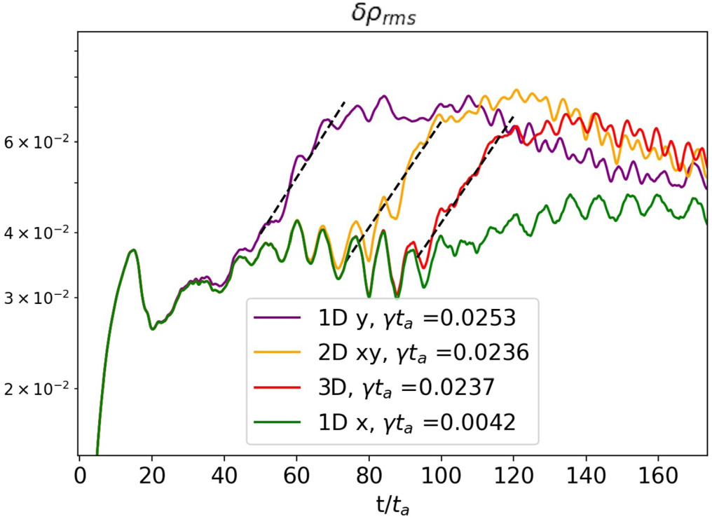
Figure 2. Evolution of the rms of δ ρ for different noise initialization. The growth rate is greatest in runs where noise in the y coordinate is present. The dashed lines show the interval over which the growth rate γ was estimated.
Download figure:
Standard image High-resolution imageBecause the wave packet is a function of (x,z), small perturbations are generated numerically in the plane containing the kink. Therefore, adding a noise that depends on x- and/or z-coordinates did not affect the decay of the wave packet. This was verified by a comparison of the growth of the density fluctuations between a simulation with no noise δ ρ0 = 0, 1D noise δ ρ0 = δ ρ0(x) or δ ρ0 = δ ρ0(z), and 2D noise δ ρ0 = δ ρ0(x, z). There was no discernible difference in the evolution of these runs, so Figure 2 only shows the 1D (x) case.
For cases where noise has a y-dependence (the invariant direction of the initial condition), unstable modes with a defined wavevector ky ≠ 0 develop. Growth rates for the ky > 0 modes are comparable regardless of the dimension of the noise, the only difference being the onset time of the linear growth phases, as shown in Figure 2. In particular, the onset of the ky > 0 linear growth phases is delayed in the 2D (x−y) and 3D cases compared to the 1D (y). Del Zanna et al. (2001) found a similar delay in the secondary decay process of monochromatic, large-amplitude circularly polarized waves across 1D, 2D, and 3D simulations. They attribute this delay to increased competition with other eigenmodes, as increasing the dimensionality of the system increases the number of degrees of freedom available (Del Zanna et al. 2001). Likewise, we attribute the delay seen here to an increase in the time it takes for the unstable eigenmodes to be selected. As we will discuss later, the growth of these modes, which require an explicit noise in the invariant direction y to be destabilized, can significantly affect the stability of the Alfvén wave packet.
Through this investigation, it was determined that initializing simulations with 1D noise in the y-direction was sufficient to investigate the full range of possible instabilities, in particular, the nature of the ky modes, and to establish baseline growth rates.
3. Results
Figures 3(a) and (b) show the evolution of the total cross helicity (σ) and of the kinetic (ek ), magnetic (em ), and internal (eth) energies for the runs considered in this work as a function of the normalized time t/tA, where tA = lx /VA is the Alfvén time of the kink. The cross helicity is defined as

with

the brackets 〈·〉 denoting spatial averaging over the simulation domain. The kinetic, magnetic, and internal energy are given, respectively, by

Because we use different box sizes while maintaining a similar or the same size of the kinked packet, we averaged over a volume of  with the switchback in the center in all the runs.
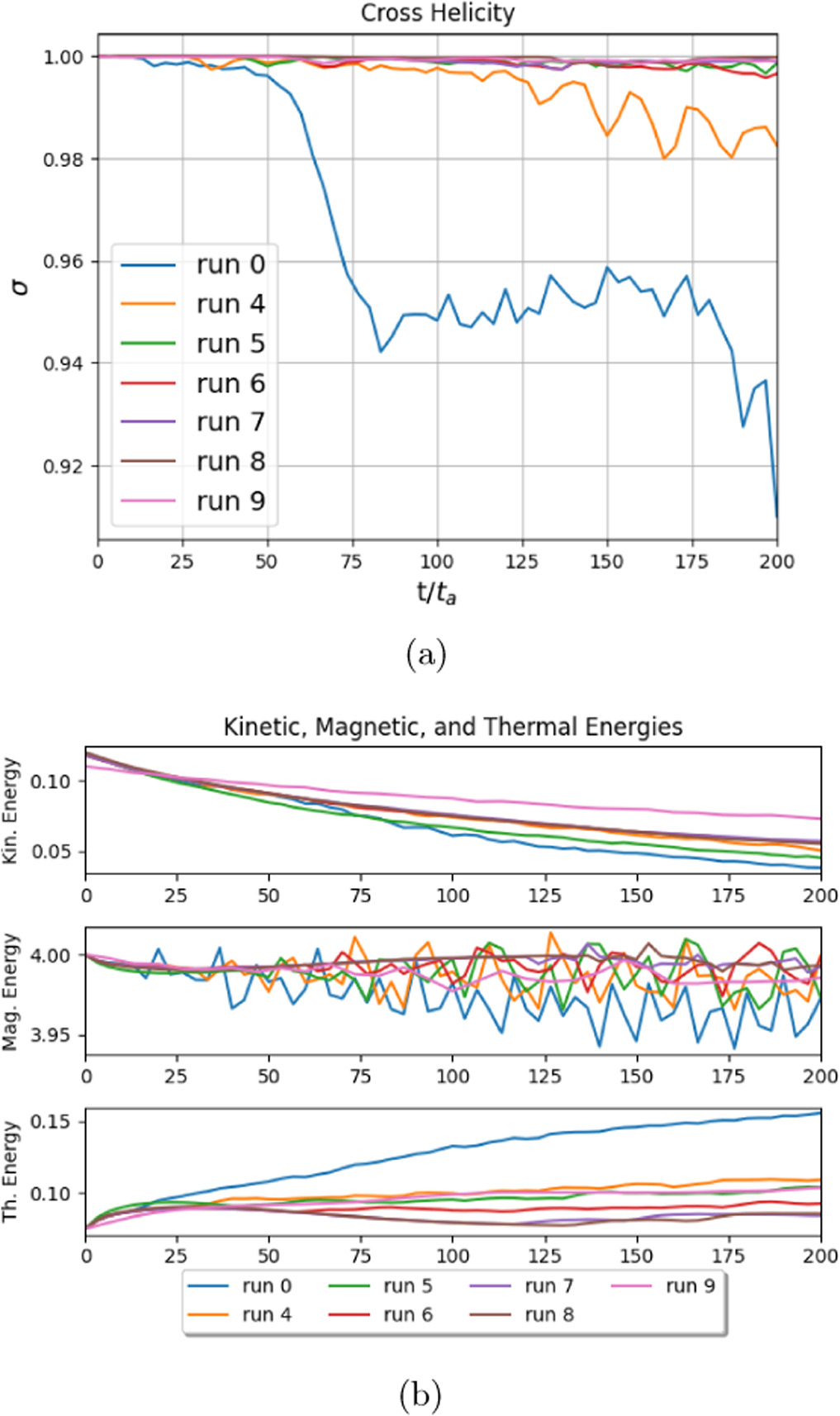
Figure 3. Cross helicity and energy profiles for the simulations listed in Table 1. Run 0 is the reference case, runs 4–8 have increasing box sizes in the direction of the propagation of the wave packet, and run 9 has a larger aspect ratio. Energy transfer is greatest for run 0, where the box size is the smallest.
Download figure:
Standard image High-resolution imageThe development of the decay of the initial wave packet is marked by a drop in the cross helicity σ, which is plotted for runs 0, 4–9 in Figure 3(a). The drop is most pronounced for run 0, which has the shortest box length. Because the cross helicity was calculated as a global parameter for a box around the wave packet, the value stays close to 1 on average. However, outside the wave packet, there are areas that develop σ ≈ −1, showing where reflected waves are generated. The decay leads to a transfer of kinetic and magnetic energy stored in the wave packet into internal energy through coupling with compressible modes, as will be discussed below. For reference, we show the time evolution of kinetic, magnetic, and internal energy for runs 0, 4–9 in Figure 3(b).
In the following sections, we first discuss the nature of the unstable modes leading to the decay by focusing on run 0. Then, we discuss how these modes and their growth rates vary with box length Lx , the effect of the aspect ratio, and the role of the propagation angle.
3.1. 3D Effects: The Reference Case (Run 0)
Because our initial condition is broadband in the (x, z) plane and invariant with respect to y, we investigate the decay process of our initial wave packet by distinguishing the growth of perturbations with wavevectors ky = 0 and ky (1), ky (2) for the modes in y with wavenumbers ny = 1, 2. (Wavevectors are related to the wavenumber by the relation k = 2π n/L.) In the following, we will refer to modes with ky = 0 and ky ≠ 0 as in-plane and transverse modes, respectively.
Figure 4 shows the time evolution of δ
ρrms in black, and colored lines correspond to the mean amplitudes of the density Fourier modes  for ky
(0) (blue), ky
(1) (orange), and ky
(2) (green), averaged over the x−z plane. As can be seen, there are two distinguishable phases of growth of the total δ
ρrms, labeled "Phase I" and "Phase II" in the plot. Phase I coincides with the growth of the ky
= 0 mode (in-plane), and corresponds to the decay observed in previous work where a 2D simulation box was considered (Tenerani et al. 2020). Phase II is instead determined by the growth of the transverse modes, which develop because of 3D effects. Growth rates of δ
ρrms for the two phases are labeled γ1 and γ2, respectively, are shown in the legend in Figure 4.
for ky
(0) (blue), ky
(1) (orange), and ky
(2) (green), averaged over the x−z plane. As can be seen, there are two distinguishable phases of growth of the total δ
ρrms, labeled "Phase I" and "Phase II" in the plot. Phase I coincides with the growth of the ky
= 0 mode (in-plane), and corresponds to the decay observed in previous work where a 2D simulation box was considered (Tenerani et al. 2020). Phase II is instead determined by the growth of the transverse modes, which develop because of 3D effects. Growth rates of δ
ρrms for the two phases are labeled γ1 and γ2, respectively, are shown in the legend in Figure 4.

Figure 4. The linear growth phases for run 0 (Lx
= 8π), showing both δ
ρrms (left vertical axis) and the growth of the first three Fourier modes,  with ny
= 0, 1, 2 (right vertical axis), plotted in a log-linear scale. The dashed lines denote the range over which the best fit was taken, yielding the γ
ta
values reported in Table 1.
with ny
= 0, 1, 2 (right vertical axis), plotted in a log-linear scale. The dashed lines denote the range over which the best fit was taken, yielding the γ
ta
values reported in Table 1.
Download figure:
Standard image High-resolution image3.1.1. In-plane Modes
The linear phase of growth for the in-plane modes occurs roughly between t/tA = 20 and t/tA = 50, and is the initial driver of the decay of the Alfvén wave packet. To capture the growth of such in-plane modes in Fourier space, we set ny = 0, average in z, and finally take the Fourier transform in x to look at the Fourier spectrum in kx .
Although our wave packet is broadband and not circularly polarized, we can interpret the in-plane dynamics in terms of the traditional theory of parametric decay (Derby 1978). We indeed observe the development of compressible modes propagating parallel to the background, guiding magnetic field along the x-axis. By using a dispersion solver, we find that the fastest-growing compressible modes predicted by linear theory have wavevector k = 1.75 for our value of the plasma beta and for an estimated relative amplitude 〈δ B〉/B0 = 0.5, with the average taken in a box around the wave packet. Accordingly, we see modes at kx = 1.75 in the Fourier spectrum of the density, as shown in Figure 5 (similar results are found for runs 4–9). They grow during the linear phase, and dominate the spectrum thereafter.
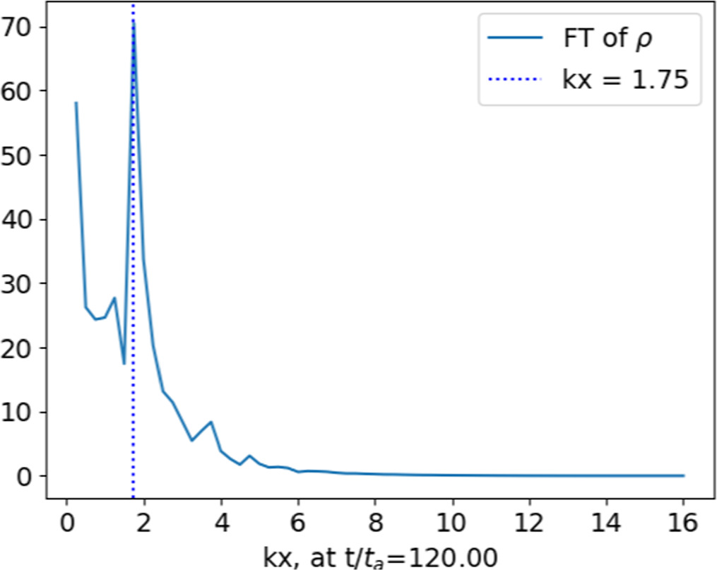
Figure 5. The solid blue line denotes the Fourier spectrum of ρ averaged in z with ny = 0 (to discount transverse modes) at 120 Alfvén times. The spectrum peaks at kx = 1.75, indicated by the dashed indigo line.
Download figure:
Standard image High-resolution image3.1.2. Transverse Modes
Previous numerical and theoretical work has shown that Alfvén waves, in either parallel or oblique propagation, can also decay by resonating with compressible modes propagating transverse to the propagation direction of the pump wave (Del Zanna 2001; Del Zanna et al. 2015). Here, we report that transverse resonant modes, previously unobserved in 2D simulations of the kinked wave, form in 3D when noise is initiated in the direction transverse to the kink, and how the formation of these modes affects the overall decay of the wave packet.
Modes with wavenumbers ny > 0 grow at a faster rate than the ny = 0 modes, although in general, the amplitude of these modes is smaller. In the Lx = 8π (run 0) case, resonance in the y-direction mainly involves Alfvén and compressible modes with wavenumbers ny = 1 and 2. These modes are visible in the x−y contour plot of the density in Figure 6 during their times of growth.

Figure 6. Contour plot of the density in the x−y plane, showing the ky (2) mode (run 0).
Download figure:
Standard image High-resolution imageWe identified the nature of the unstable transverse modes by looking at the correlation between the velocity, magnetic, and density fields, shown in Figure 7. To help the analysis, we averaged fields with respect to the x- and z-coordinates. In this way, we identify three dominant modes that obey the aforementioned resonant condition that can be easily identified because the mean field is predominantly along the y-axis: a fast mode propagating backward mostly in y with ny = 1, characterized by positively correlated fluctuations δ ux and δ Bx , shown in the top panel of Figure 7; an Alfvén mode propagating backward in y with ny = 1, with positively correlated δ uz and δ Bz is shown in the second panel; and a slow mode is shown in the bottom panel, propagating forward in y with ny = 2, with positively correlated δ ρ and δ uy .
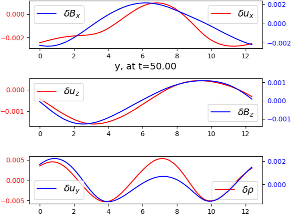
Figure 7. δ Bx and δ ux are correlated, showing that the fast mode with ky = 1 propagates backward. δ Bz and δ uz are correlated, showing an Alfvén mode with ky = 1 that also propagates backward. Finally, δ uy and δ ρ are correlated with ky = 2 for the slow mode.
Download figure:
Standard image High-resolution imageWe further calculated the amplitude ratio of the Fourier coefficients, namely, the ratio δ uy (ky )/δ ux (ky ) for ky (1) and ky (2) and compared it with the values for fast and slow modes predicted from the linearized MHD system, assuming a homogeneous plasma with a mean magnetic field forming an angle of 69° from the x-axis (as in our simulation). The predicted velocity ratios are δ uy (ky )/δ ux (ky ) = 0.38 for the fast mode and δ uy (ky )/δ ux (ky ) = 2.64 for the slow mode, in agreement with theory. This allows us to confirm that, indeed, ky (2) is the slow mode, while the fast mode is ky (1).
3.2. System Size Effects
The switchback interacts with past perturbations as they cycle through the periodic box, as illustrated in Figure 8, where the colored scale represents Bx contours, and the black and white contour lines represent the density. The compressible density disturbance generated by our kinked magnetic field, in particular, stands out in black and white, and the periodic interaction with this disturbance contributes to the decay of the wave packet. We performed simulations of several increasing Lx in order to investigate the impact of this effect, and in Figure 9, we report the inferred growth rates of parametric decay for our runs 0, 4–8.
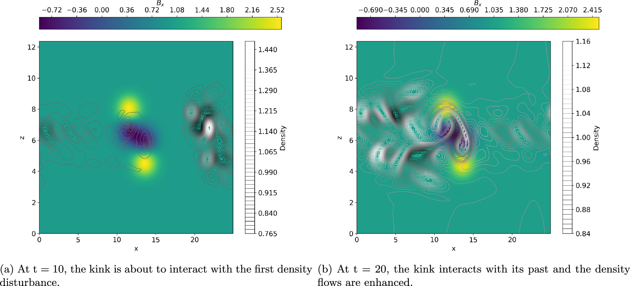
Figure 8. The x-component of the magnetic field is shown in the yellow to blue color scale, overlapped with a contour line plot of the density in gray scale in the x−z plane. The density shows a kinked shape within the negative region of the magnetic field.
Download figure:
Standard image High-resolution image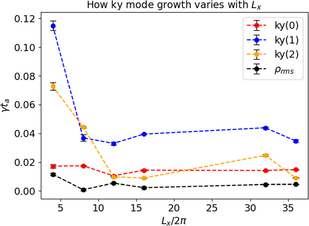
Figure 9. Growth rates for δ ρrmsrms (black) and the ky modes, plotted against box length (runs 0, 4–8), Lx in units of 2π.
Download figure:
Standard image High-resolution image
Figure 10. The minimum value of Bx over time for runs 0, 4–8, which have increasing box length. The periodicity seen in runs 4–8 comes from the wave packet interacting with the initial density fluctuation as it travels through the periodic box. These interactions can push the magnetic field to negative values even after Bx (min) has been positive.
Download figure:
Standard image High-resolution imageThe δ ρrms growth rate (γ) generally decreases with increasing Lx , in line with expectations from Tenerani et al. (2020). However, when the box size becomes much larger than the wave packet length, Lx ≫ lx , the growth rate of the in-plane and transverse modes is only weakly affected by the box size. We argue that as the growth rates decrease and unstable modes require more time to fill larger boxes, the actual growth rate of unstable modes falls below detectable levels, and the growth of density fluctuations is mainly determined by initial transients, as also found, for example, in Malara et al. (2000). We also note that as the box size increases, the ny = 1 mode remains the dominant transverse mode, uncoupled from higher wavenumber modes. However, its growth is delayed and its amplitude remains small, so the effect this mode has on the overall δ ρrms is negligible at long box lengths. The timing of the onset of the unstable modes varied, rather inconsistently, so that our separation of the effect of the transverse modes from the in-plane modes into two phases, as was done for run 0, was not a valid paradigm for all runs.
Unfolding Switchback. A negative value of Bx , meaning that the magnetic field has a component pointing opposite to the direction of propagation, a key signature used to identify the largest amplitude switchbacks among data obtained from spacecraft. Therefore, in order to estimate the total time it takes for our kink to unfold, we looked at the minimum value of Bx . When Bx (min) was no longer negative, we considered the switchback to be unfolded. The time it takes to unfold, we refer to as τlife, the lifetime of the switchback.
Figure 10 shows the evolution of Bx (min) over time for runs varying in box length. The switchback for the Lx = 8π case has a consistently, nearly linear progression of Bx (min) and reaches 0 at about 230 Alfvén times. Larger box sizes displayed a periodicity in the progression of Bx (min). The kink generates an initial density fluctuation, which it interacts with after traveling the length of the box (see Figure 8). The peaks of Bx (min) occur when the kink interacts with this initial fluctuation, and so this periodicity is determined by the time it takes the wave packet to cross one box length.
This periodic behavior shows that the kink can reform (e.g., Bx (min) can return to negative values after reaching positive values) during interactions with other density fluctuations that squish and pull its shape. Such interactions would be common in the solar wind, and these results suggest that switchbacks are robust as they travel through the solar wind. Despite these oscillations in Bx , generally τlife increases with increasing box length. The effect of system size, however, decreasingly affects the dynamics of the wave packet as the box length increases.
3.3. Aspect Ratio
Changing the aspect ratio, lx /lz , also requires changing the set amplitude, ψ0, in order to preserve an overall similar shape to the original run. So we set lx = 3 and ψ0 = 1.5, which gives us a magnetic field very similar to the original run, still with θ ∼ 69° and B ∼ 3.23. Since the ratio lx /Lx significantly affects the growth rate, we impose a box length of Lx = 16π, so that the lx /Lx ratio is the same as that for run 0. With these changes, the growth of the transverse modes was negligible, while the growth rate for the ky (0) mode increased to about 1.5 times the rate of run 0 (see Table 1). However, overall, the lifetime estimate of run 9 was 230 Alfvén times, about the same amount of time as run 0. We also find that the aspect ratio affects the growth of the transverse modes. The ny = 2 mode does not grow, but the wavenumber is still conserved in this case by the development of two pairs of ny = 1 modes: a forward and a backward fast mode, and a forward and a backward Alfvén wave. However, the growth of these modes is slower with respect to run 0, and their amplitude remains negligible compared to the in-plane modes.
3.4. Propagation Angle and Amplitude
Run 10 corresponds to a smaller amplitude wave packet in quasi-parallel propagation with respect to the mean field. The angle θ to the x-axis, in this case, is θ = 35°, and the amplitude is ψ0 = 0.25. The quasi-parallel case had slower dynamics than the quasi-perpendicular case, due to its smaller amplitude, such that the box length had to be shortened to Lx = 4π in order to speed up the evolution.
Even in this quasi-parallel setup, we still see strong growth of modes in the transverse direction. In Figure 11, we see a drop in the cross helicity prior to t ∼ 500, and then it increases again. The initial drop in cross helicity coincides with the first phase of δ ρrms growth (see Figure 12), and consequently the energy transfer from kinetic and magnetic energy to thermal energy. This phase is driven entirely by the transverse modes, with ky (2) dominating. The cross helicity then takes a turn and increases again, marking a secondary decay process. During this time, the in-plane modes (ky (0)) grow, and ky (1) replaces ky (2) as the dominant transverse mode.
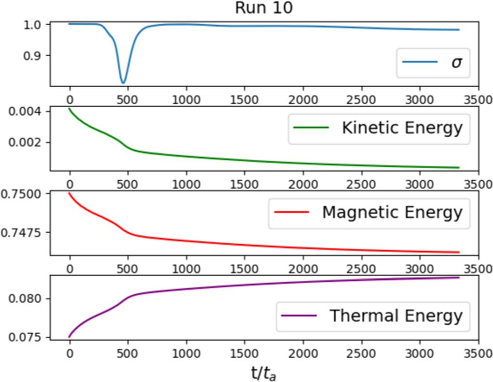
Figure 11. The cross helicity and energy profiles in time for run 10. A drop in the cross helicity marks the first parametric decay phase, and the sharp increase shortly afterward suggests a secondary decay.
Download figure:
Standard image High-resolution image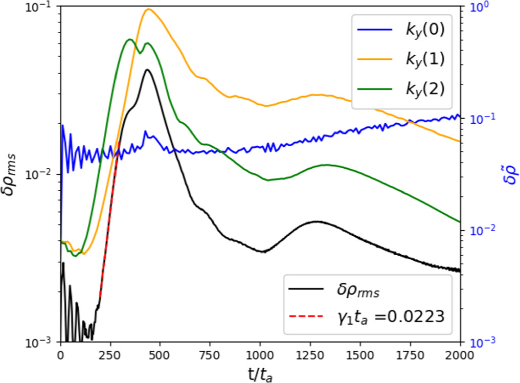
Figure 12. The δ ρrms (left vertical axis) and ky modes (right vertical axis) for run 10. The transverse modes grow first, with the ky (0) modes developing later at a much slower pace. The δ ρrms largely follows the development of the transverse modes.
Download figure:
Standard image High-resolution image
By inspecting the dynamics of fields in the y-direction during the linear phase, we find that Alfvén and compressible modes have grown, this time with ny = 2 dominating for all modes. As in the other runs, we see both forward- and backward-propagating Alfvén waves, each with ny = 2, and two magnetosonic waves, one forward and one backward, each with ny = 2.
The magnetic field has no negative components in this initial setup. Although the criteria of Bx
(min) used for the larger amplitude kink is not applicable in this case, we looked at how the amplitude of the variance  changed over time, specifically
 ![$\left[\delta {B}_{x}{\left(t\right)}^{2}-\delta {B}_{x}^{2}(0)\right]/\delta {B}_{x}^{2}(0)$](https://content.cld.iop.org/journals/0004-637X/967/1/19/revision1/apjad38b9ieqn13.gif) , to quantify how the wave packet is decaying. We find that after a time of about 675 Alfvén times
, to quantify how the wave packet is decaying. We find that after a time of about 675 Alfvén times  has decreased by 50%. The period of steepest decrease lasts until about 900 Alfvén times, encapsulating the first and secondary decay processes seen in the cross helicity and the rise and fall of the transverse modes. After about t = 1000, during the slow growth of the parallel modes,
  continues to decrease but at a markedly slower pace.
We conclude that the development of transverse modes is not dependent on a large propagation angle, and the decay takes place, although over longer timescales, even for such a small amplitude wave packet.
4. Summary and Discussion
We have investigated the dynamics of a kinked, localized Alfvén wave packet with a 3D periodic MHD code. In analogy with past work, we find that the initial wave packet decays by coupling with compressible and Alfvénic modes due to parametric instability. The localization of the wave packet has a strong stabilizing effect on the decay, and we find that increasing the box size decreases the growth rate, in agreement with 2D simulations by Tenerani et al. (2020). There is a minimum growth rate reached, which may represent the minimum growth rate of parametric decay in an infinite box. However, it is perhaps more likely that other competing processes, such as transients, establish this minimum, and the true growth rate due to parametric decay becomes too small to be detected at large box lengths.
Transverse Mode Growth. In contrast to the previous studies with 2D simulations, modeling the full 3D dynamics allows the growth of unstable modes in the invariant direction (y) of the initial kinked structure (thus, transverse to the propagation direction).
Because our model initially lacks gradients in the y-direction, these transverse modes only grow when random noise fluctuations are initialized in that direction. These modes are destabilized even for wave packets of smaller amplitude and in quasi-parallel propagation, and with larger aspect ratio. However, the growth rate of transverse modes is affected. The larger aspect ratio case was less stable (run 9 versus run 0), with a slightly higher growth rate for the in-plane modes despite a slower growth rate for the transverse modes, suggesting that the compactness of the wave packet affects its stability. The smaller amplitude case, predictably, was much more stable (run 10 versus run 0), with lower growth rates of both the in-plane and transverse modes.
Although the growth of transverse modes can speed up the decay process, in contrast to when they are not allowed to form (as in 2D), we still find that the wave packet survives slightly longer in the 3D box than in a 2D box (230 versus 200 Alfvén times, according to Tenerani et al. 2020). This is because the onset of the parametric instability is delayed in 3D simulations when compared to 2D or 1D simulations, as found in previous work (Del Zanna et al. 2001).
Implications for the Stability of Switchbacks in the Solar Wind. We can obtain an order-of-magnitude estimate of the radial distance traversed by our wave packet using the formula ΔR = τlife(vw + vA), where τlife is the amount of time (in seconds) it takes for the wave packet to decay.
We assume an average solar wind speed of vw ≃ 150 km s−1 and an average Alfvén speed of vA ≃ 500 km s−1, between R ≃ 1 and ≃30 R⊙. With a length scale of lx
= 5 × 10⁴ km, typical of a switchback (Laker et al. 2020), we obtain that the Alfvén time is roughly lx
/vA = tA = 100 s. Then, by taking the results for the Lx
= 8π case, which is the most unstable one, we find ΔR ≃ 21 R⊙, just slightly longer than the 2D case. For run 6, which had the longest τlife and Lx
= 32π, the distance roughly doubles to ΔR ≃ 43R⊙. Note that, by using the fact that τlife = α
ta
where α is a coefficient,  . The estimated distance traveled by a switchback is, thus, sensitive to the (1) size of the switchback lx
and (2) ratio of the solar wind speed to the Alfvén speed. Larger scale switchbacks in faster streams are expected to reach longer radial distances.
. The estimated distance traveled by a switchback is, thus, sensitive to the (1) size of the switchback lx
and (2) ratio of the solar wind speed to the Alfvén speed. Larger scale switchbacks in faster streams are expected to reach longer radial distances.
Energy Conversion during Switchback Decay. We estimate the contribution of a decaying switchback to the internal energy of the solar wind by taking typical values of density and temperature at R ≃ 0.3 au (Hellinger et al. 2011). We assume n0 ≃ 25 cm−3 and T0 ≃ 6 × 10⁵ K, an Alfvén time of 100 s, and evaluate the energy change over the initial Δt = 200 ta for all runs in order to be consistent. Then, for run 0, Δeth tA/(Δteth(0)) ≃ 0.5%, and we get that the internal energy increases at the rate of Δeth/Δt ≃ 1.7 × 10⁻¹⁴ Wm−3. Predictably, the heating rate decreases with increasing box size. In run 8 (Lx = 72π), Δeth tA/(Δteth(0)) ≃ 0.07%, leading to an estimate of Δeth/Δt ≃ 2.1 × 10⁻¹⁵ Wm−3, which is the same order of magnitude as the observational estimate. The smallest amplitude wave packet considered exhibited the weakest increase in internal energy, Δeth tA/(Δteth(0)) ≃ 0.017%, in line with expectations that larger amplitude wave packets can transfer more energy to internal energy (Tenerani et al. 2023).
Finally, in our simulations, the internal energy increases because of wave energy conversion mediated by the generation of compressible modes. Despite the generation of counter-propagating Alfvénic modes, the system does not develop a turbulent cascade, and the magnetic energy spectra remain steep, with a slope of nearly  ,
,  , and
, and  . This suggests that the decay of a wave packet cannot be the sole source of the observed turbulent cascade; however, coupling of Alfvén fluctuations with compressible modes can contribute to increasing solar wind internal energy.
Limitations of the Model and Conclusions. In this work, we have considered a two-dimensional Alfvénic wave packet. Therefore, our model is applicable in the case where the wave packet is highly anisotropic in one direction, such that its size in one direction is much larger than the wavelength of the most unstable modes. Therefore, our results are valid as long as the length of the switchback in y, ly is much larger than the wavelength of the dominant mode in that direction, i.e., λ = 2π/ky0. In our simulation box, the wavelength of the ny = 1 mode is λ = 4π, i.e., the length of the box in Ly . With lx = 1.5, the ratio is then ly /lx = 8.37. It would not be unreasonable to expect that in cases where ly /lx > 10, initial gradients in y can be neglected.
Although we have adopted a simplified model for a switchback, our results support the idea that it is possible that some switchbacks are generated close to the solar corona. These structures evolve as they propagate in the inner heliosphere and eventually decay. Here, we have shown that the parametric decay instability is one possible mechanism by which switchbacks decay by converting their energy into plasma internal energy. Our results also suggest that not only solar wind conditions, such as speed and underlying turbulence, but also the structure of the wave packet itself has an impact on the stability of switchbacks. Depending on their size, other effects not included in this study may, however, come into play, such as dispersive effects (Tenerani et al. 2023) and underlying gradients (Magyar et al. 2021), which can disrupt the initial kink faster than parametric decay; and velocity shears, which instead, may help to maintain it (Toth et al. 2023). Inclusion of some of these physical effects will be included in future work.
Acknowledgments
This research was supported by The NSF Graduate Research Fellowship Program under grant No. DGE 2137420 and the NSF CAREER award 2141564. The authors also acknowledge the Texas Advanced Computing Center (TACC) at The University of Texas at Austin for providing HPC resources that have contributed to the research results reported within this paper. 1 Any opinions, findings, conclusions, or recommendations expressed in this material are those of the authors and do not necessarily reflect the views of the National Science Foundation.