


Abstract
We present the second and final release of optical spectroscopy of Type Ia supernovae (SNe Ia) obtained during the first and second phases of the Carnegie Supernova Project (CSP-I and CSP-II). The newly released data consist of 148 spectra of 30 SNe Ia observed in the course of CSP-I and 234 spectra of 127 SNe Ia obtained during CSP-II. We also present 216 optical spectra of 46 historical SNe Ia, including 53 spectra of 30 SNe Ia observed by the Calán/Tololo Supernova Survey. We combine these observations with previously published CSP data and publicly available spectra to compile a large sample of measurements of spectroscopic parameters at maximum light, consisting of pseudo-equivalent widths and expansion velocities of selected features for 232 CSP and historical SNe Ia (including more than 1000 spectra). Finally, we review some of the strongest correlations between spectroscopic and photometric properties of SNe Ia. Specifically, we define two samples: one consisting of SNe Ia discovered by targeted searches (most of them CSP-I objects) and the other composed of SNe Ia discovered by untargeted searches, which includes most of the CSP-II objects. The analyzed correlations are similar for both samples. We find a larger incidence of SNe Ia belonging to the cool and broad-line Branch subtypes among the events discovered by targeted searches, shallow-silicon SNe Ia are present with similar frequencies in both samples, while core normal SNe Ia are more frequent in untargeted searches.
Export citation and abstract BibTeX RIS

Original content from this work may be used under the terms of the Creative Commons Attribution 4.0 licence. Any further distribution of this work must maintain attribution to the author(s) and the title of the work, journal citation and DOI.
1. Introduction
The number of observational studies of Type Ia supernovae (SNe Ia) has continually increased as a result of their great importance to multiple fields of astrophysics. For example, SNe Ia are the primary source of iron-peak elements in the Universe, and their energy input plays an important role in the heating of interstellar matter in galaxies. They also provide important constraints on binary evolution in the Galaxy. But, probably their most outstanding property is that they are excellent extragalactic distance indicators, e.g., Zwicky et al. (1961), and thus powerful tools for the determination of the cosmological expansion rate as a function of look-back time (e.g., Burns et al. 2018; Freedman 2021; Khetan et al. 2021; Riess et al. 2022; Uddin et al. 2023).
The Carnegie Supernova Project (CSP) began taking data in 2004 with the expressed goal of obtaining high-precision optical and near-infrared photometry of a large sample of SNe Ia acquired in well-understood photometric systems in order to characterize the ultimate precision of these events for determining distances (Hamuy et al. 2006). During its first phase (CSP-I), which operated for 5 yr between 2004 and 2009, light curves were obtained for 123 nearby SNe Ia (Contreras et al. 2010; Stritzinger et al. 2011; Krisciunas et al. 2017). A large number of optical spectra were also acquired for these SNe Ia, 604 of which were published by Folatelli et al. (2013). During a second phase of the project (CSP-II), carried out between 2011 and 2015, optical and near-infrared photometry were obtained for 214 SNe Ia, 125 of which were located in the smooth Hubble flow at redshifts of 0.027 < z < 0.137 (Phillips et al. 2019). A major goal of CSP-II was to obtain near-infrared spectroscopy, and more than 650 such spectra were acquired from 157 SNe Ia (Hsiao et al. 2019). A significant number of optical spectra were also obtained, many for classification purposes, while more extensive follow-up was performed for a limited number of events.
In this data release paper, we present 148 previously unpublished optical spectra of 30 SNe Ia observed during the course of CSP-I and 234 previously unpublished spectra of 127 SNe Ia observed during CSP-II. The CSP-I spectra presented here were not included in Folatelli et al. (2013) because at the time of the publication of that paper, definitive photometry was not yet available for the corresponding objects, and as a consequence, the analysis of spectroscopic and photometric properties could not be carried out in the same way as for the other SNe Ia. CSP optical spectra have already been published for SN 2010ae (Stritzinger et al. 2014), SN 2011iv (Gall et al. 2018), SN 2012Z (Stritzinger et al. 2015), SN 2012fr (Childress et al. 2013), iPTF13ebh (Hsiao et al. 2015), SN 2013gy (Holmbo et al. 2019), ASASSN-14lp (Shappee et al. 2016), LSQ14fmg (Hsiao et al. 2020), ASASSN-15hy (Lu et al. 2021), SN 2015bp (Wyatt et al. 2021), SN 2007if, SN 2009dc, LSQ12gpw, SN 2013ao, CSS140501-170414+174838 and SN 2015M (Ashall et al. 2021), and SN 2015bo (Hoogendam et al. 2022). Also, a large number of CSP optical spectra of SNe Ia obtained near maximum light have been analyzed by Burrow et al. (2020) using Gaussian mixture models. The approach in this paper differs from the latter in that we intend to derive spectroscopic parameters at the time of maximum light for the SNe Ia in our sample, and only those objects for which such parameters were obtained are considered in the discussion that follows.
In addition, we include in this paper a number of spectra of what we shall refer to as historical SNe Ia. These consist of the following:
- 1.53 optical spectra of 30 SNe Ia observed by the Calán/Tololo Supernova Survey (Hamuy et al. 1993).
- 2.163 optical spectra of an additional 16 SNe Ia were obtained mostly by members of the Calán/Tololo team. Several of these spectra have been included in previous publications: SN 1986G (Phillips et al. 1987), SN 1989B (Wells et al. 1994), SN 1991T (Phillips et al. 1992), SN 1991bg (Leibundgut et al. 1993), SN 1992A (Kirshner et al. 1993), and SN 1992K (Hamuy et al. 1994), but are not yet publicly available on WISeREP (Yaron & Gal-Yam 2012). Some of the spectra were acquired during the execution of the Supernova Optical and Infrared Survey (PI: M. Hamuy, 1999–2000; Hamuy 2001; Hamuy et al. 2002a, 2002b).
The primary goal of this paper is to make these 598 optical spectra available to the community. We combine them with the 604 CSP-I spectra published by Folatelli et al. (2013) and the previously published CSP-I and CSP-II optical spectra mentioned above to reexamine some of the correlations between spectral and photometric properties presented by these authors. Results for the SNe Ia drawn from targeted searches are compared with those discovered in untargeted (blind) searches. Incorporated in this new analysis is the color stretch parameter sBV (Burns et al. 2014), which is more effective at characterizing the fastest-declining SNe Ia than the widely used Δm15(B) parameter (Phillips 1993). Note that all the newly presented data, including spectra of CSP I and II targets and the historical SNe Ia, will be released electronically via WISeREP.
The outline of this paper is as follows: in Section 2, the different spectroscopic data sets are detailed; in Section 3, measurements of expansion velocities and pseudo-equivalent widths (pWs) are presented along with notes on a few specific SNe; in Section 4, we reexamine some of the spectroscopic and photometric correlations derived by Folatelli et al. (2013) using the measurements presented in this paper, augmented by those of the SNe Ia published by these authors; finally, in Section 5 a brief summary of the results is given.
2. Data
Summaries of the new observations, classifications, and photometric properties of the SNe Ia considered in this paper are presented in Table 1 (for CSP-I and CSP-II data) and Table 2 (for the historical SNe Ia). Photometric parameters for the CSP I and II targets are taken from Uddin et al. (2023). For the historical SNe Ia, template light-curve fits were computed using SNooPy (Burns et al. 2011) to the available photometry of our objects retrieved from the references given in the final column of Table 2.
Table 1. Summary of Observations, Spectroscopic, and Photometric Properties of CSP SNe Ia Considered in This Work
| SN | N | Phase Range | SNID | Wang | Branch | zHelio | t(max) | Δm15 | sBV |
|---|---|---|---|---|---|---|---|---|---|
| (day) | (MJD) | (mag) | |||||||
| (1) | (2) | (3) | (4) | (5) | (6) | (7) | (8) | (9) | (10) |
| CSP-I | |||||||||
| 2005gj | 18 | 38.0, 341.4 | Ia-CSM | ⋯ | ⋯ | 0.0616 | 53657.30(1.28) a | ⋯ | ⋯ |
| 2007if b | ⋯ | 6.5, 30.5 | Ia-pec (SC) | Normal | SS | 0.0742 | 54348.4 c | ⋯ | ⋯ |
| 2007jd | 5 | 14.4, 44.3 | Normal | HV | BL | 0.0726 | 54361.9(1.0) | 1.304(0.065) | 0.891(0.054) |
| 2007ol | 7 | −3.5, 20.1 | Normal | Normal | CN | 0.0559 | 54412.9(0.2) | 1.576(0.068) | 0.701(0.051) |
| 2007so | 5 | 22.5, 41.0 | Normal | ⋯ | ⋯ | 0.0297 | 54428.0(0.5) | 1.196(0.067) | 0.925(0.041) |
| 2007st | 6 | 6.7, 35.9 | Normal | ⋯ | ⋯ | 0.0212 | 54454.4(0.7) | 1.428(0.081) | 0.863(0.046) |
| 2008O | 3 | 0.5, 28.4 | Normal | HV | CL | 0.0389 | 54491.8(0.6) | 1.617(0.061) | 0.688(0.041) |
| 2008ae | 4 | 0.6, 28.7 | Ia-pec | ⋯ | ⋯ | 0.0300 | 54508.63(0.60) d | 1.648(0.078) | ⋯ |
| 2008bd | 4 | 7.6, 13.5 | 91bg-like | 91bg | ⋯ | 0.0301 | 54531.2(0.5) | 1.785(0.072) | 0.660(0.055) |
| 2008bi | 6 | 9.8, 47.2 | 91bgi-like | 91bg | ⋯ | 0.0134 | 54543.3 (0.9) | 1.977 (0.073) | 0.512 (0.046) |
Notes. Column (1): SN designation. Column (2): number of spectra released in this work. Ellipsis means that we are not presenting new spectroscopic observations of the target, but based on previously published spectra, we include it in the discussion of SN properties at maximum light. Column (3): phases (expressed in days) of the first and last spectra. Column (4): SNID classification. Column (5): Wang subtype. Column (6): Branch subtype. Column (7): heliocentric redshift of the host. The adopted redshift for LSQ12hnr is discussed in Section 3.3. Column (8): MJD of B maximum light from the SNooPy fit when available. Column (9): Δm15 (in magnitudes) from the SNooPy fit when available. Column (10): color stretch sBV from SNooPy fit when available. For the data in columns (8)–(10), errors are given in parentheses.
a t(max) derived from g-band light curve (Prieto et al. 2007). b 03fg-like (Ashall et al. 2021). c t(max) from Scalzo et al. (2010). d t(max), Δm15, and sBV are derived from the observed light curves instead of SNooPy fits. e Observed during the course of CSP, but not included in the final sample. f Phase estimated using SNID. g t(max) from Marion et al. (2016). h t(max) from Singh et al. (2018).Only a portion of this table is shown here to demonstrate its form and content. A machine-readable version of the full table is available.
Download table as: DataTypeset image
Table 2. Summary of Observations, Spectroscopic, and Photometric Properties of Historical SNe Ia
| SN | N | Phase Range | SNID | Wang | Branch | zHelio | t(max) | Δm15 | sBV | Photometry |
|---|---|---|---|---|---|---|---|---|---|---|
| (day) | (MJD) | (mag) | ||||||||
| (1) | (2) | (3) | (4) | (5) | (6) | (7) | (8) | (9) | (10) | (11) |
| 1981B | ⋯ | ⋯ | Normal | HV | BL | 0.0060 | 44671.5 | 1.10(0.07) | ⋯ | |
| 1986G | 17 | −6.1, 55.8 | 91bg | 91bg | CL | 0.0018 | 46561.192(0.077) | 1.420(0.025) | 0.602(0.012) | 1 |
| 1989B | 59 | −8.2, 345.3 | Normal | Normal | BL | 0.0024 | 47565.377(0.180) | 1.053(0.011) | 0.883(0.010) | 2 |
| 1990N | 7 | −14.0, 37.6 | Normal | Normal | SS | 0.0033 | 48082.208(0.040) | 0.931(0.009) | 1.147(0.008) | 3 |
| 1990O | 6 | −7.4, 19.6 | Normal | Normal | CN | 0.0303 | 48075.945(0.171) | 0.905(0.012) | 1.107(0.032) | 4 |
| 1990T a | 4 | 14.5, 34.7 | Normal | ⋯ | ⋯ | 0.0404 | 48083.068(0.210) | 1.066(0.008) | 0.985(0.017) | 4 |
| 1990Y a | 1 | 19 | Normal | ⋯ | ⋯ | 0.0360 | 48114.129(0.612) | 1.035(0.023) | 1.099(0.067) | 4 |
| 1990af a | 2 | −3.6,−3.6 | 91bg | 91bg | CN | 0.0506 | 48195.867(0.120) | 1.516(0.021) | 0.744(0.009) | 4 |
| 1991S a | 1 | 18.5 | Normal | ⋯ | ⋯ | 0.0546 | 48346.883(0.361) | 0.918(0.017) | 1.096(0.061) | 4 |
| 1991T | 20 | −8.9, 338.8 | 91T | 91T | SS | 0.0070 | 48374.999(0.128) | 0.801(0.015) | 1.212(0.009) | 3 |
Notes. The descriptions of the columns are as in Table 1. SNooPy fits are available for all SN other than 1993af and 1999cs. References for the photometry: (1) Phillips et al. (1987); (2) Wells et al. (1994); (3) Lira et al. (1998); (4) Hamuy et al. (1996); (5) Leibundgut et al. (1993); (6) N. B. Suntzeff (2024, in preparation); (7) Strolger et al. (2002); (8) Lennarz et al. (2012); (9) Hamuy et al. (2002a); (10) Krisciunas et al. (2004a); (11) Krisciunas et al. (2004b).
a Calán/Tololo Supernova Survey. b Phase estimated using SNID.Only a portion of this table is shown here to demonstrate its form and content. A machine-readable version of the full table is available.
Download table as: DataTypeset image
In the successive columns of Tables 1 and 2, we list the supernova (SN) identification; the number of new spectra released in this work (three dots mean that no new spectra are presented); the phase range covered by them; the SN classification obtained from running SNID (Blondin & Tonry 2007) on the earliest spectrum available to us; the Wang et al. (2009) subtype; the Branch et al. (2006) subtype; the heliocentric redshift 44 of the host as listed in Krisciunas et al. (2017) and Phillips et al. (2019) except for LSQ12hnr, discussed in Section 3.3; the time of maximum light; and the decline rate (Δm15) 45 and color stretch (sBV) parameters from SNooPy fits (unless otherwise specified).
Journals of the spectroscopic observations, including details about the telescopes and instruments used, are presented in Tables 3 and 4 for the CSP and historical SNe Ia, respectively.
Table 3. CSP Optical Spectra of SNe Ia Considered in This Work
| Date | Date | Phase | Tel. | Inst. | λ Range | Res. | Exp. | Airmass | Rms |
|---|---|---|---|---|---|---|---|---|---|
| (UT) | (MJD) | (day) | (Å) | (Å) | (s) | ||||
| (1) | (2) | (3) | (4) | (5) | (6) | (7) | (8) | (9) | (10) |
| CSP-I | |||||||||
| SN 2005gj | |||||||||
| 2005:11:24.2 a | 53698.2 | 38.0 | DUP | MS | 3780–7290 | 7.0 | 3 × 900 | 1.15 | 0.163 |
| 2005:11:25.2 | 53699.2 | 39.0 | DUP | MS | 3780–7290 | 7.0 | 3 × 900 | 1.15 | 0.054 |
| 2005:12:18.2 | 53722.2 | 60.7 | NTT | EM | 3400–5300 | 6.0 | 3 × 300 | 1.45 | 0.053 |
| 2005:12:18.2 | 53722.2 | 60.7 | NTT | EM | 4000–10200 | 9.0 | 3 × 300 | 1.61 | ⋯ |
| 2005:12:18.2 | 53722.2 | 60.7 | NTT | EM | 5800–10200 | 9.0 | 3 × 300 | 1.80 | ⋯ |
| 2005:12:20.2 | 53724.2 | 62.5 | DUP | WF | 3800–9235 | 8.0 | 3 × 900 | 1.21 | 0.034 |
| 2005:12:21.1 | 53725.1 | 63.4 | DUP | WF | 3800–9235 | 8.0 | 3 × 900 | 1.25 | 0.049 |
| 2005:12:22.2 | 53726.2 | 64.4 | DUP | WF | 3800–9235 | 8.0 | 3 × 1200 | 1.32 | 0.040 |
| 2005:12-23.2 | 53727.2 | 65.3 | DUP | WF | 3800–9235 | 8.0 | 3 × 1200 | 1.38 | 0.039 |
| 2005:12:24.2 | 53728.2 | 66.3 | DUP | WF | 3800–9235 | 8.0 | 3 × 1200 | 1.41 | 0.038 |
| 2006:01:16.1 | 53751.1 | 87.9 | NTT | EM | 3400–5300 | 6.0 | 3 × 300 | 1.30 | 0.040 |
| 2006:01:16.1 | 53751.1 | 87.9 | NTT | EM | 4000–10200 | 9.0 | 3 × 300 | 1.39 | ⋯ |
| 2006:01:16.1 | 53751.1 | 87.9 | NTT | EM | 5800–10200 | 9.0 | 3 × 300 | 1.49 | ⋯ |
| 2006:01:24.1 | 53759.1 | 95.4 | CLA | LD | 3788–6134 | 2.0 | 900 | 1.57 | 0.038 |
| 2006:01:24.1 | 53759.1 | 95.5 | CLA | LD | 5778–10000 | 4.0 | 900 | 1.87 | ⋯ |
| 2006:03:05.0 | 53799.0 | 133.0 | DUP | WF | 3800–9235 | 8.0 | 1200 | 1.78 | ⋯ |
| 2006:09:27.2 | 54005.2 | 327.3 | DUP | WF | 3800–9235 | 8.0 | 3 × 1800 | 1.24 | ⋯ |
| 2006:10:12.2 | 54020.2 | 341.4 | DUP | WF | 3800–9235 | 8.0 | 3 × 1800 | 1.14 | ⋯ |
Notes. Column (1): UT date of the observation. Column (2): modified Julian Date. Column (3): phase in days relative to the time of maximum light corrected for redshift. Column (4): telescope code. 3P6: ESO 3.6 m Telescope at La Silla; BAA: Las Campanas Magellan I 6.5 m Baade Telescope; CLA: Las Campanas Magellan II 6.5 m Clay Telescope; DUP: Las Campanas 2.5 m du Pont Telescope; GEN: Gemini-N 8 m Telescope; GES: Gemini-S 8 m Telescope; NTT: ESO New Technology Telescope at La Silla; NOT: Nordic Optical Telescope at Roque de los Muchachos, Canary Islands. Column (5): instrument code. AL: Alhambra Faint Object Spectrograph and Camera (ALFOSC); BC: Boller & Chivens spectrograph; EF: ESO Faint Object Spectrograph and Camera (EFOSC-2); EM: ESO Multi-Mode Instrument (EMMI); GM: Gemini Multiple-Object Spectrograph (GMOS); IM: Inamori Kyocera Magellan Areal Camera and Spectrograph (IMACS); LD: Low Dispersion Survey Spectrograph (LDSS); MA: Magellan Echellette spectrograph (MagE); MI: Magellan Inamori Kyocera Echelle spectrograph (MIKE); MS: Las Campanas Modular Spectrograph (MODSPEC); WF: Wide Field Reimaging CCD Camera (WFCCD). Column (6): observed spectral range expressed in angstrom. Column (7): spectral resolution in angstrom. Column (8): exposure time in seconds. Column (9): airmass at the middle of the exposure. Column (10): rms of the differences between synthetic and observed broadband magnitudes (when available).
a Spectrum corrected to match photometry. b Phase estimated using SNID. c Spectrum not corrected for telluric absorption.Only a portion of this table is shown here to demonstrate its form and content. A machine-readable version of the full table is available.
Download table as: DataTypeset image
Table 4. Optical Spectroscopic Observations of Historical SNe Ia
| Date | Date | Phase | Tel. | Inst. | λ Range | Exp. | Airmass |
|---|---|---|---|---|---|---|---|
| (UT) | (MJD) | (day) | (Å) | (s) | |||
| (1) | (2) | (3) | (4) | (5) | (6) | (7) | (8) |
| SN 1986G | |||||||
| 1986:05:05.1 | 46555.1 | −6.1 | C60 | RC60 | 4787–7179 | ⋯ | ⋯ |
| 1986:05:06.1 | 46556.1 | −5.1 | C60 | RC60 | 4787–7179 | ⋯ | ⋯ |
| 1986:05:07.0 | 46557.0 | −4.2 | C60, BLA | RC60, RC4 | 3600-7154 | ⋯ | ⋯ |
| 1986:05:08.1 | 46558.1 | −3.2 | C60, BLA | RC60, RC4 | 3600-7162 | ⋯ | ⋯ |
| 1986-05:09.0 | 46559.0 | −2.2 | BLA | RC4 | 3600–5171 | ⋯ | ⋯ |
| 1986:05:10.2 | 46560.2 | −1.0 | BLA | RC4 | 3918–7018 | ⋯ | ⋯ |
| 1986:05:11.3 | 46561.3 | 0.1 | BLA | RC4 | 3556–6638 | ⋯ | ⋯ |
| 1986:05:12.2 | 46562.2 | 1.0 | BLA | RC4 | 3556–6638 | ⋯ | ⋯ |
| 1986:05:13.1 | 46563.1 | 1.9 | BLA | RC4 | 3698–5265 | ⋯ | ⋯ |
| 1986:-05:15.4 | 46565.4 | 4.2 | H88 | ⋯ | 4374–6330 | ⋯ | ⋯ |
| 1986:05:17.0 | 46567.0 | 5.8 | BLA | RC4 | 5991–7012 | ⋯ | ⋯ |
| 1986:-06:09.5 a | 46590.5 | 29.3 | YAL | YBC | 3800–7218 | ⋯ | ⋯ |
| 1986:06:25.0 | 46606.0 | 44.8 | YAL | YBC | 3800–7218 | ⋯ | ⋯ |
| 1986:06:27.1 | 46608.1 | 46.9 | DUP | DBC | 4600–7200 | ⋯ | ⋯ |
| 1986:06:29.0 | 46610.0 | 48.8 | YAL | YBC | 3800–7218 | ⋯ | ⋯ |
| 1986:07:04.0 | 46615.0 | 53.8 | YAL | YBC | 3800–7218 | ⋯ | ⋯ |
| 1986:07:06.0 | 46617.0 | 55.8 | DUP | DBC | 3300–7100 | ⋯ | ⋯ |
Notes. Column (1): UT date of observation. Column (2): modified Julian Date. Column (3): phase in days relative to maximum light corrected for redshift. Column (4): telescope code. BLA: CTIO 4.0 m Blanco Telescope; C60: Cerro Tololo Inter-American Observatory (CTIO) 1.5 m Telescope; DUP: Las Campanas 2.5 m du Pont Telescope; H88: U. Hawaii 2.2 m Telescope; K84: Kitt Peak National Observatory (KPNO) 2.1 m Telescope; MMT: Multiple Mirror Telescope (MMT) at the Fred Lawrence Whipple Observatory; NIC: Lick Observatory 1.0 m Nickel Telescope; NOT: Nordic Optical Telescope at Roque de los Muchachos, Canary Islands; NTT: ESO New Technology Telescope at La Silla; SHA: Lick Observatory 3.0 m Shane Telescope; TIL: 1.5 m Tillinghast Telescope at the Fred Lawrence Whipple Observatory; YAL: CTIO 1.0 m Yale Telescope; 1P5: ESO 1.5 m Telescope at La Silla; 3P6: ESO 3.6 m Telescope at La Silla. Column (5): instrument code. AL: Alhambra Faint Object Spectrograph and Camera (ALFOSC); DBC: Las Campanas 2.5 m Boller & Chivens spectrograph; EBC: ESO 1.5 m Boller & Chivens spectrograph; EF: ESO Faint Object Spectrograph and Camera (EFOSC-2); EM: ESO Multi-Mode Instrument (EMMI); GOLD: Gold Camera; RC4: CTIO 4.0 m R-C Spectrograph; RC60: CTIO 1.5 m R-C Spectrograph; RED: Red Channel; WF: Wide Field Reimaging CCD Camera (WFCCD); YBC: Yale 1.0 m Boller & Chivens spectrograph; ZM: Z-Machine; CS1: Lick 1.0 m Cassegrain Spectrograph; CS3: Lick 3.0 m Cassegrain Spectrograph. Column (6): observed spectral range in angstrom. Column (7): exposure time in seconds. Column (8): airmass at the middle of the observation. Spectra already available via WISeREP are not included in this table, although they are considered in the analysis of SN properties at maximum light that follows.
a This spectrum is the sum of spectra taken on 1986 June 8 and 1986 June 11. b Phase estimated using SNID. c This spectrum has a gap between 4870 and 5100 Å.Only a portion of this table is shown here to demonstrate its form and content. A machine-readable version of the full table is available.
Download table as: DataTypeset image
The optical spectra obtained by the CSP Collaboration were reduced using standard IRAF 46 routines as described in Hamuy et al. (2006). Briefly, reductions included bias subtraction, flat fielding, wavelength calibration with arc lamp exposures obtained right before or after the SN observation, and flux calibration with spectra of spectrophotometric standard stars observed during the same night as the science targets. In the vast majority of the cases, the slit was oriented according to the parallactic angle. A few exceptions were made when the parallactic orientation would result in a bright host nucleus significantly contaminating the SN spectrum. At least one telluric standard chosen from Bessell (1999) was also observed during each observing night with the same slit width as that used for the SN observation in order to correct for telluric absorption features. When a telluric standard spectrum was not obtained on the same night as the science observations, no telluric correction was attempted. Such spectra are labeled as not corrected for telluric absorption in Table 3.
The spectra obtained with the GMOS instrument on Gemini were reduced following standard procedures with the IRAF Gemini/GMOS package.
Optical spectra taken with the Nordic Optical Telescope (NOT) were obtained using ALFOSC (Andalucia Faint Object Spectrograph and Camera) with grism 4. Data reduction of NOT spectra was performed following standard procedures using a set of custom MatLab scripts written by F. Taddia. Flux calibration was performed using sensitivity functions derived from observations of the standard star(s) obtained on the same night as the science observations.
As in Folatelli et al. (2013), in the last column of Table 3, we provide the rms of the differences between two or more synthetic magnitudes calculated from the spectra and observed magnitudes in the same filters interpolated to the exact time of the spectral observation from the CSP light curves, after removal of a constant flux term. This number provides a measure of the correctness of the shape of the flux-calibrated spectrum. In some cases, we were not able to perform this comparison, either due to the restricted wavelength coverage of the spectrum, or because the photometric data did not cover the epoch of the spectrum. When the rms was larger than ∼0.15 mag for at least three bandpasses, we used a low-order polynomial function to correct the overall shape of the spectrum.
Most of the spectra of the historical SNe Ia were also calibrated using standard IRAF routines. Unfortunately, for some of these observations, details of the exposure time, airmass, and in a few cases, the instrument used have been lost. No attempt has been made to quantify errors in the shapes of the spectra introduced in the flux calibration through comparison with available photometry.
3. Measurements
3.1. Expansion Velocities and pWs
We measured expansion velocities and pWs of selected features as described in Folatelli et al. (2013). Following the definitions in Garavini et al. (2007; see Figure 4 and Table 5 of Folatelli et al. 2013) we performed measurements of the following features: Ca ii H&K (pW1), Si ii λ4130 (pW2), Mg ii λ4481 (pW3; blended with Fe ii and dominated by Ti ii in the Branch CL class), Fe ii at ∼4600 Å (pW4, blended with S ii), the S ii "W" feature at ∼5400 Å (pW5), Si ii λ5972 (pW6), Si ii λ6355 (pW7), and the Ca ii "IR triplet" (pW8).
All measurements were made by means of the IRAF splot task from the onedspec package. Line expansion velocities were derived from Gaussian fitting of the minimum of each absorption trough. The pW measurements were obtained by direct integration between two defined pseudo-continuum positions. Error estimates were computed with splot setting the number of samples for error computation (the nerrsample parameter) to 100, the sigma0 parameter (uniform component of the uncertainty) to the rms flux measured in the nearby pseudo-continuum, and disregarding any Poissonian component of the uncertainty (i.e., setting the invgain parameter to zero). We adopted 1 Å as the minimum realistic uncertainty for pW measurements. For some critical features, such as Si ii λ5972, when unable to obtain a reliable measurement because the feature was very weak or not detected, we estimated upper limits of pW considering the signal-to-noise ratio in the spectral region where such a feature would be expected.
3.2. Spectroscopic Parameters at Maximum Light
The measurements described above for our own spectra were analyzed in combination with similar measurements of spectra of the targets in Table 1, which are publicly available through WISeREP, specifically when our observations were not sufficiently close to maximum light to compute the desired spectroscopic parameters. The procedure followed is the same as that described in Folatelli et al. (2013) and is summarized as follows:
- 1.In cases where several spectra encompassing maximum light were available to us, we fit low-order polynomials to our pW and expansion velocity measurements and used those functions to interpolate the values at maximum.
- 2.When two spectra were available in the interval −4 to +4 days from maximum, we interpolated values at maximum from them.
- 3.If only data before or after maximum were available, but one spectrum was obtained within 1 day of maximum light, an extrapolation was allowed.
- 4.In the most frequent cases where only one spectrum was available within the range −4 to +4 days from maximum, we applied the slopes given in Tables 4 and 7 of Folatelli et al. (2013) to estimate values at maximum light, combining the errors estimated for our measurements with those coming from the assumed slopes.
This procedure allowed the determination of pWs and expansion velocities at maximum light for the selected features in 15 CSP I SNe Ia not included in our previous spectroscopic release (Folatelli et al. 2013), 113 SNe Ia observed by CSP II, and 27 historical SNe Ia. All targets for which we were able to derive spectroscopic parameters at maximum light are included, regardless of their being considered as normal or peculiar SNe Ia. The values of the pWs at maximum light are presented in Table 5. Measurements of expansion velocities at maximum light can be found in Table 6. Note that the SNe are sorted by Branch type (Branch et al. 2006) in both tables.
Table 5. pWs at Maximum Light (Angstrom)
| SN | pW1 | pW2 | pW3 | pW4 | pW5 | pW6 | pW7 | pW8 | Project |
|---|---|---|---|---|---|---|---|---|---|
| Ca ii H&K | Si ii 4130 | Mg ii | Fe ii | S ii W | Si ii 5972 | Si ii 6355 | Ca ii IR | ||
| CN | |||||||||
| 2007ol | 106(1) | 22(1) | 80(1) | 82(1) | 56(1) | 16(1) | 78(1) | ⋯ | CSP-I |
| 2008bz | 86(2) | 22(2) | 70(1) | 106(2) | 88(1) | 17(1) | 99(1) | 105(3) | CSP-I |
| 2008fr | 107(2) | 11(1) | 71(2) | 109(1) | 80(1) | 17(1) | 82(2) | 72(5) | CSP-I |
| 2009I | 140(3) | 9(1) | 82(3) | 111(2) | 72(1) | 10(1) | 70(1) | 89(3) | CSP-I |
| 2009cz | 120(1) | 9(1) | 92(1) | 131(1) | 67(1) | 12(1) | 81(1) | 104(4) | CSP-I |
| 2009le | 60(2) | 11(1) | 104(2) | 124(1) | 62(1) | 9(1) | 86(1) | 114(2) | CSP-I |
| ASASSN-14hr | 135(2) | 32(1) | 101(2) | 138(1) | 67(2) | 30(1) | 104(2) | 107(4) | CSP-II |
| ASASSN-14hu | 150(2) | 11(1) | 97(2) | 115(1) | 76(1) | 7(1) | 83(1) | ⋯ | CSP-II |
| ASASSN-14kq | 139(1) | 11(1) | 100(1) | 115(1) | 73(1) | 11(1) | 77(1) | 127(3) | CSP-II |
| ASASSN-14lp | 116(3) | 10(1) | 93(4) | 140(3) | 69(1) | 13(1) | 70(1) | 117(4) | CSP-II |
Note. All pW values and their errors (in parentheses) are expressed in angstrom.
Only a portion of this table is shown here to demonstrate its form and content. A machine-readable version of the full table is available.
Download table as: DataTypeset image
Table 6. Expansion Velocities at Maximum Light and Si ii 6355 Velocity Decline (Kilometers per Second)
| SN | Ca ii H&K | Si ii 4130 | S ii 5449 | S ii 5622 | Si ii 5972 | Si ii 6355 | Ca ii IR | Δv20(Si) | project |
|---|---|---|---|---|---|---|---|---|---|
| CN | |||||||||
| 2007ol | 17,110(212) | 11,217(98) | 9822(258) | 9365(222) | 11,546(244) | 11,577(195) | ⋯ | 1559(331) | CSP-I |
| 2008bz | 15,632(266) | 10,534(27) | 8883(58) | 8992(47) | 10,704(72) | 11,303(39) | 9710(257) | 1253(151) | CSP-I |
| 2008fr | 12,296(141) | 10,175(95) | 9940(436) | 9208(117) | 10,709(198) | 11,098(118) | 12,239(335) | ⋯ | CSP-I |
| 2009I | 12,000(187) | 9764(84) | 9296(136) | 9696(94) | 9959(147) | 10,768(79) | 12,169(192) | 675(165) | CSP-I |
| 2009cz | 18,359(65) | 8448(60) | 8270(136) | 8086(99) | 9560(192) | 9697(78) | 17,545(248) | ⋯ | CSP-I |
| 2009le | 12,570(247) | 12,259(51) | 10,495(145) | 10,948(65) | 11,071(181) | 12,654(66) | 12,273(396) | ⋯ | CSP-I |
| ASASSN-14hr | 17,242(140) | 10,650(70) | 8783(125) | 8527(137) | 11,083(182) | 11,747(306) | 11,905(251) | ⋯ | CSP-II |
| ASASSN-14hu | 13,054(191) | 10,634(27) | 9797(63) | 10,047(35) | ⋯ | 11,511(36) | ⋯ | 1143(89) | CSP-II |
| ASASSN-14kq | 12,573(214) | 9165(82) | 8626(192) | 9067(82) | 10,000(223) | 10,584(112) | 10,482(271) | ⋯ | CSP-II |
| ASASSN-14lp | 11,605(103) | 11,356(259) | 10,526(127) | 10,790(266) | 12,499(246) | 11,982(303) | 16772(656) | 693(303) | CSP-II |
Note. Velocities and their error estimates (in parentheses) are expressed in kilometers per second.
Only a portion of this table is shown here to demonstrate its form and content. A machine-readable version of the full table is available.
Download table as: DataTypeset image
3.3. Notes on Particular Targets
LSQ12ca. This SN Ia has the lowest value of Δm15 in the CSP-II sample (0.618 ± 0.081 mag), although its sBV (1.195 ± 0.097), while high, is comparable to that of other normal SNe Ia. From the spectrum available to us, obtained at phase 2.8 days past maximum, we derive normal values for its expansion velocities and pWs at maximum light. C ii absorption is probably present on the red side of the Si ii λ6355 line.
LSQ12gpw. There are three public spectra of this SN Ia from PESSTO, 47 available in WISeREP: the one obtained at phase −1.5 days and the other two at phase −0.5 day. There is also one CSP spectrum at phase +5.8 days. All these spectra show an absorption line, redward of Si ii λ6355, well separated from the Si ii feature that, if identified as C ii λ6580, yields expansion velocities of approximately 7500, 7400, and 6200 km s−1, for phases −1.5, −0.5, and +5.8 days, respectively.
LSQ12hno shows expansion velocities somewhat lower than usual (∼8000–9000 km s−1) in our two spectra obtained at 2.4 and 1.5 days before maximum light, respectively.
LSQ12hnr. Two spectra of LSQ12hnr are available in WISeREP, both obtained by PESSTO, at phases +0.8 and +10.8 days, respectively. The classification report by Le Guillou et al. (2012) gave a possible redshift of z = 0.135 inferred from the SN Ia spectrum. No obvious host is detected in our follow-up images or in a deep, Very Large Telescope (VLT)-MUSE observation of the SN Ia site. However, an apparent cluster of galaxies is observed whose brightest member lies about 40'' west of the SN Ia location. We determined redshifts for the three brightest galaxies in that cluster (from a total of at least four), obtaining a weighted average of z = 0.1243 ± 0.0002, the value we therefore adopted for LSQ12hnr assuming this SN Ia occurred in a fainter member of the same cluster of galaxies.
OGLE-2013-SN-015. There is only one CSP spectrum of this SN Ia, which, albeit noisy, seems normal, and was obtained very close to maximum light (phase = +0.7 days). However, our photometric follow-up was poor for this target, and consequently, we decided not to consider this SN Ia in our analysis of SN properties at maximum light.
OGLE-2013-SN-123. There is only one spectrum available from WISeREP, obtained by the PESSTO Collaboration at maximum light, which shows clear evidence of host galaxy contamination, and therefore, the pWs measured from it are unreliable, as well as the spectral type determined via SNID. However, we obtained a spectrum of the host galaxy with the WFCCD instrument on the Las Campanas 2.5 m du Pont telescope in 2019 to determine its redshift. By scaling the host spectrum and subtracting it from the SN Ia observation so as to make the obvious stellar Na i D blend at ∼5892 Å absorption and the TiO feature at ∼7150 Å disappear, the other stellar features such as Ca ii H&K, the G band at ∼4300 Å, Hβ, and Mg ib λ5175 also mostly disappeared (see Figure 1). We, therefore, have used this host galaxy subtracted spectrum to derive the spectroscopic properties at maximum light for this SN Ia.
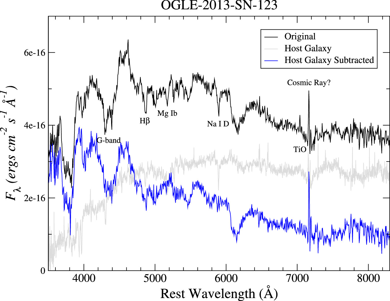
Figure 1. The spectrum of OGLE-2013-SN-123 after galaxy subtraction. The black spectrum is the original PESSTO observation, the gray spectrum is that of the host galaxy obtained by CSP-II, and the blue spectrum is the difference between the two after scaling the host galaxy spectrum to minimize the stellar features in the original PESSTO spectrum. Due to the differing wavelength resolution of the spectra, some residual subtraction features are evident (e.g., for the Na i D line). See the text for further details.
Download figure:
Standard image High-resolution imageASASSN-15eb. The classification report by Childress et al. (2015) does not refer to any peculiarities; however, SNID yields some matches with 91T-like SNe at maximum light. According to our light curve, this spectrum corresponds to phase +4.5 days. The pWs are indeed small, but this is clearly caused by strong host contamination. Also, strong Galactic Na i D absorption is evident in that spectrum. The CSP spectrum published here, obtained at phase +11.0 days, also exhibits significant host galaxy contamination as well as strong Na i D absorption from the Milky Way. Both spectra show absorption minima on the red side of Si ii λ6355, which could be attributed to C ii.
4. Results
In this section, we combine the Si ii expansion velocities and selected pW measurements from this paper with those derived by Folatelli et al. (2013) to take a second look at some of the plots and correlations discussed in that paper. In particular, our interest is to highlight agreements and differences between the properties of SNe Ia discovered in targeted versus untargeted searches.
4.1. Temporal Evolution of the Expansion Velocities of Si ii λ6355
For a limited number of CSP-II targets and historical SNe Ia, the available data span enough time to follow the evolution of the Si ii λ6355 expansion velocity to at least 20 days past maximum light. These observations are presented in the left and right panels of Figure 2, respectively, with the different Branch types indicated by the colors and shapes of the symbols. In general, albeit with less data here, the behavior observed in this figure is very similar to that of Figure 9 of Folatelli et al. (2013). In both panels, the shaded region represents the upper and lower 1σ dispersion of the Si ii λ6355 expansion velocity evolution for the whole CSP-I and II sample of Branch CN SNe with normal Wang classification subtypes (see Table 7 for details).
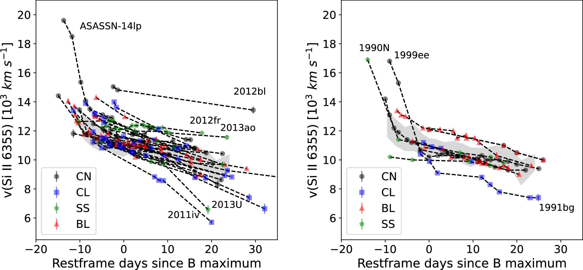
Figure 2. Temporal evolution of the expansion velocities of the Si ii λ6355 line for samples of the CSP-II targets (left) and the historical SNe Ia (right). The symbols reflect the corresponding Branch types: black-filled circles for CN, green pentagons for SS, red triangles for BL, and blue squares for CL. Error bars are plotted except when smaller than the symbols. Dashed lines connect data for each SN. In both panels, the shaded region represents the upper and lower 1σ dispersion computed for all the Branch CN SNe with normal Wang classification subtypes in the whole CSP-I and II sample.
Download figure:
Standard image High-resolution imageTable 7. Temporal Evolution of the Si ii λ6355 Expansion Velocities in the CSP-I and II Sample
| Phase | Exp. Vel. | Sigma | N | Phase | Exp. Vel. | Sigma | N | Phase | Exp. Vel. | Sigma | N | ||
|---|---|---|---|---|---|---|---|---|---|---|---|---|---|
| −9.5 | 12,449 | 869 | 9 | 1.5 | 10,950 | 451 | 29 | 13.5 | 10,261 | 600 | 5 | ||
| −7.5 | 11,861 | 886 | 16 | 3.5 | 10,706 | 494 | 20 | 15.5 | 10,319 | 665 | 6 | ||
| −5.5 | 11,437 | 802 | 17 | 5.5 | 10,805 | 468 | 6 | 19.0 | 9937 | 693 | 5 | ||
| −3.5 | 11,532 | 903 | 19 | 7.5 | 10,453 | 649 | 11 | 21.0 | 9116 | 832 | 4 | ||
| −1.5 | 11,066 | 696 | 26 | 9.5 | 10,190 | 653 | 12 | 24.0 | 9812 | 543 | 6 | ||
| 0 | 10,861 | 619 | 71 | 11.5 | 10,290 | 514 | 8 |
Note. Phase: rest-frame phase of bin center; exp.vel.: average expansion velocity; sigma: standard deviation; N: number of data in a bin.
Download table as: ASCIITypeset image
From Figure 2 (left panel), we can see that SN 2012bl shows high Si ii λ6355 velocity, which persists 29 days past maximum light, although measurements of the minimum of Si ii λ6355 after 20 days post maximum are questionable due to blending with other features. SN 2012fr (Childress et al. 2013; Cain et al. 2018; Contreras et al. 2018) is an example of flat velocity evolution, in which the expansion velocity of Si ii λ6355 is almost constant over the period covered by our data (−5.0 to +17.8 days).
For all the SNe Ia presented in this paper with sufficient time coverage, the difference between the Si ii λ6355 velocity at maximum light and at 20 days past maximum, Δv20(Si ii), was calculated using the same methodology described in Section 3.1.1 of Folatelli et al. (2013). These values are given in the last column of Table 6 and plotted in Figure 3 as a function of light-curve decline rate Δm15 and color stretch sBV, respectively, along with the CSP-I objects already presented in Folatelli et al. (2013). Figure 3 confirms the strong correlation 48 observed by Folatelli et al. (2013) between Δv20(Si ii) and Δm15 for Branch SS, CN, and CL SNe, suggesting that these events form a single sequence. On the other hand, the lack of a correlation for the Branch BL events is consistent with previous hints that these objects may represent a distinct group of SNe Ia (e.g., see Wang et al. 2013; Burrow et al. 2020).
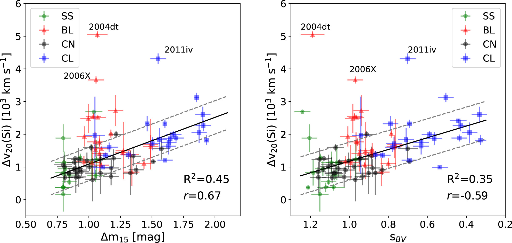
Figure 3. The left and right panels show the Si ii λ6355 velocity decline rates as a function of the light-curve decline rate Δm15 and color stretch sBV, respectively, for all the SNe Ia with sufficient phase coverage in the combined sample, which includes CSP-I, CSP-II, and historical SNe Ia. The limited number of CSP-II and historical targets for which this computation was possible causes the left panel of this figure to be very similar to Figure 21 of Folatelli et al. (2013). As found in that work, the correlation is stronger when the BL SNe Ia are excluded from the fit. Shown in both figures are the best-fit lines, intrinsic scatter lines (dotted gray), coefficients of determination (R2), and correlation coefficients (r), excluding the BL events. The transitional SN Ia 2011iv is an obvious outlier.
Download figure:
Standard image High-resolution image4.2. Correlations Involving Spectroscopic Parameters
In the analysis of spectroscopic parameters at maximum light, we consider separately the objects discovered by targeted and untargeted surveys. That is, SNe Ia in the CSP-I, CSP-II, and historical samples discovered by amateur astronomers or other targeted surveys (e.g., the Lick Observatory Supernova Survey or the Chilean Automatic Supernova Search) will be considered as one sample, while all the targets drawn from untargeted surveys such as the La Silla-QUEST (LSQ), the Palomar Transient Factory (PTF, iPTF), the Sloan Digital Sky Survey or the Catalina Real Time Transient Survey (CRTS), ASAS-SN, among others, will be considered as a second sample. The Calán/Tololo SNe are a special case since the photographic plates were taken in an untargeted fashion, but were searched for stellar objects that appeared near galaxies. We, therefore, have grouped these SNe with the targeted events. Most of the CSP-I SNe Ia belong to the targeted group and most of the CSP-II SNe Ia belong to the untargeted one. However, there are a few exceptions. CSP-II SNe Ia for which we derived spectroscopic parameters at maximum light, and that are included in the first group of targeted survey discoveries are PSN J13471211-2422171 and the SNe 2011iv, 2011jh, 2012E, 2012ah, 2012fr, 2012hd, 2012 hr, 2012ht, 2013aa, 2013fz, 2013gy, 2013hn, 2014I, 2014Z, 2014ao, 2014at, 2014dn, 2014eg, and 2015F. On the other hand, CSP-I targets for which we present spectroscopic parameters at maximum light that were discovered by untargeted searches are SNe 2007if, 2007ol, 2008bz, and 2008fr.
4.3. The Branch Diagram
Figure 4 displays the Branch et al. (2006) diagram for the targeted (left) and untargeted (right) samples of CSP and historical SNe Ia. In defining the boundaries between the four classes (CN = "core normal," SS = "shallow silicon," BL = "broad lined," CL = "cool"), we follow the definitions adopted by Folatelli et al. (2013). The largest difference between these diagrams is for the BL SNe Ia, whose relative numbers are clearly different. To be precise, the BL SNe Ia represent 31% ± 5% of the targeted sample, but only 13% ± 4% of the untargeted events. This difference is explained by the fact that targeted searches are biased toward luminous galaxies, and high-velocity SNe Ia (approximately two-thirds of which belong to the BL class) are known to occur preferentially in luminous galaxies (Wang et al. 2013). Similarly to the BL events, CL SNe—those with relatively large values of pW6 (Si ii 5972)—represent 21% ± 4% of the targeted and 15% ± 4% of the untargeted samples, respectively. As for the CN SNe, they are more frequent in the untargeted sample, amounting to 50% ± 9% of the total, compared to 33% ± 6% of the targeted sample. The SS SNe, which correspond to the classical 1991T-like and 1999aa-like events, show a less significant difference, amounting to 22% ± 5% of the untargeted sample, while in the targeted sample, they represent 15% ± 4%. These percentages are illustrated for the targeted and untargeted samples, respectively, in Figure 5. For further comparison, we show in Figure 6 histograms of our pW6 and pW7 measurements at maximum light for the untargeted and targeted samples, separately for each of the Branch types.
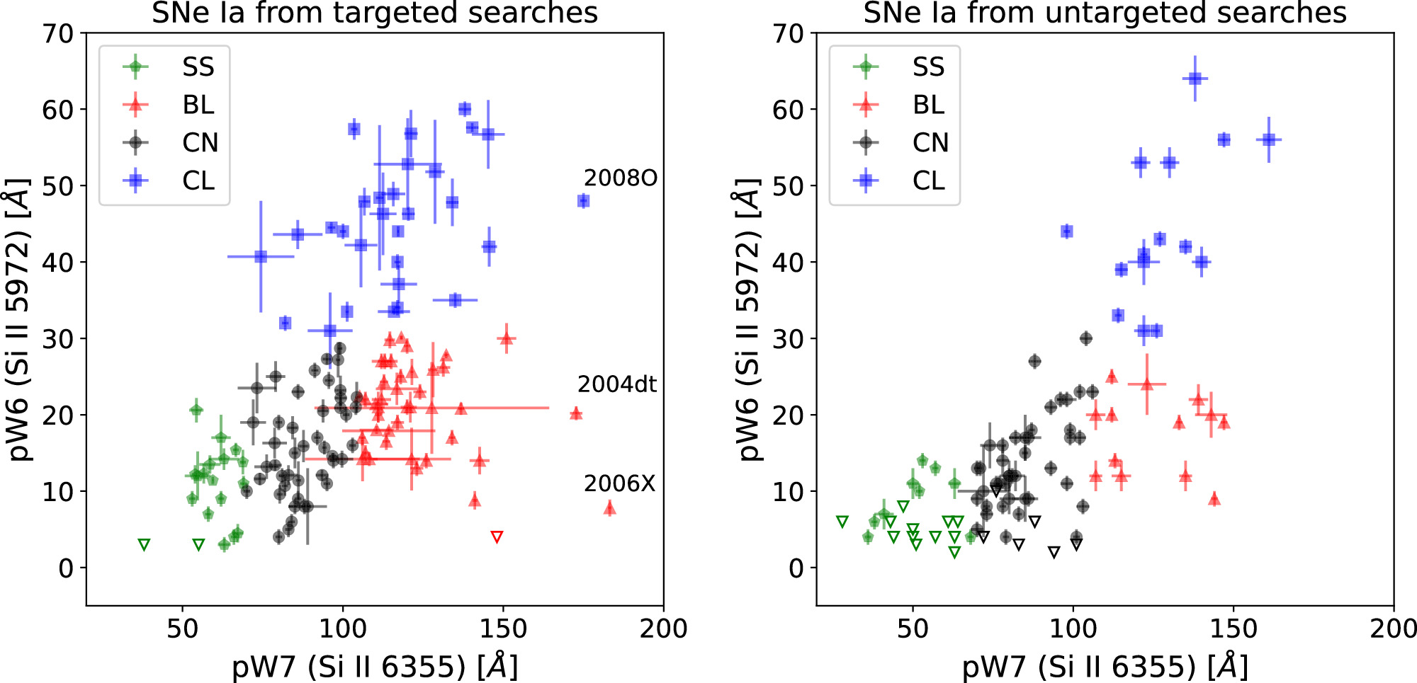
Figure 4. Branch diagrams for our two different samples. Left: historical SNe Ia and CSP-I + II SNe Ia discovered during targeted surveys (45 CN, 29 CL, 42 BL, and 20 SS SNe Ia). Right: CSP-I + II SNe Ia from untargeted surveys (48 CN, 15 CL, 13 BL, and 21 SS SNe Ia). The meaning of the symbols is as follows: black dots represent CN SNe Ia; green pentagons represent SS SNe Ia; red triangles represent BL SNe Ia, and blue squares represent CL SNe Ia. Open symbols represent upper limits.
Download figure:
Standard image High-resolution image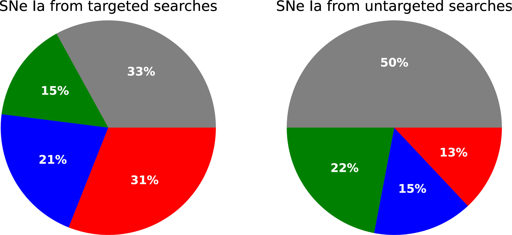
Figure 5. Pie charts showing the incidence of the different Branch types of SNe Ia in our targeted and untargeted samples, respectively.
Download figure:
Standard image High-resolution image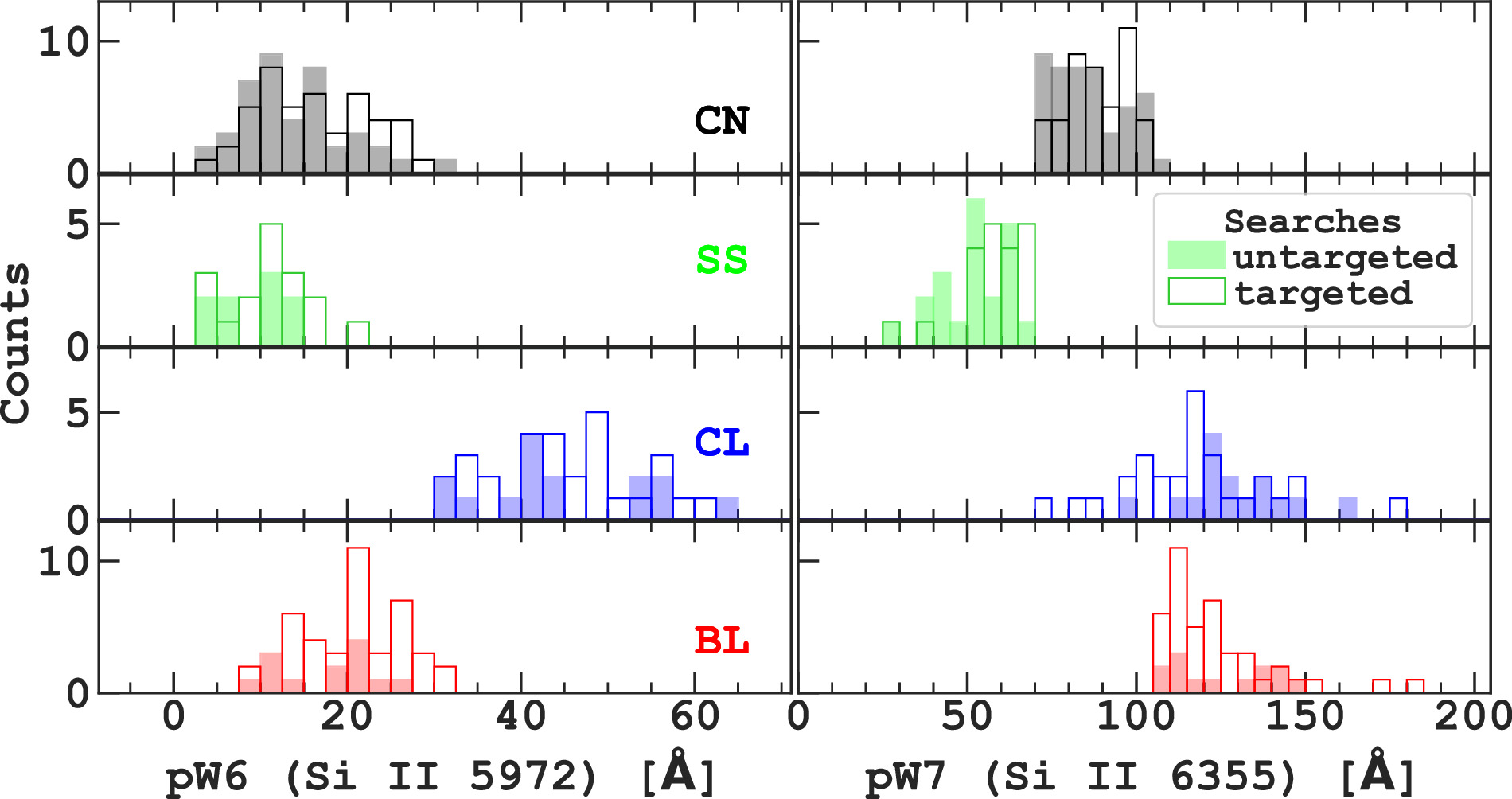
Figure 6. Histograms showing the distribution of the measured pW6 and pW7 separately for each Branch type. Colored and empty bars represent untargeted and targeted searches, respectively.
Download figure:
Standard image High-resolution imageAnother way to look at these numbers is to consider ratios. In particular, how do the ratios of the numbers of SS, CL, and BL SNe Ia compare to the number of CN SNe Ia for the targeted and untargeted samples? In the case of the targeted SNe, N(SS)/N(CN) = 0.44, N(CL)/N(CN) = 0.64, and N(BL)/N(CN) = 0.93, while for the untargeted events we find N(SS)/N(CN) = 0.44, N(CL)/N(CN) = 0.31, and N(BL)/N(CN) = 0.27. These numbers imply that SS SNe Ia are equally common with respect to CN SNe in targeted versus untargeted surveys. On the other hand, CL SNe Ia are twice as common and BL SNe are more than three times more common with respect to CN SNe in targeted surveys compared to untargeted surveys. This likely reflects the fact that SS and CN SNe Ia occur in hosts over a large range of luminosity, whereas CL and BL SNe Ia prefer luminous hosts (e.g., see Neill et al. 2009; Wang et al. 2013; Pan 2020).
Note that Burrow et al. (2020) explored the Branch diagram through a cluster analysis instead of using predefined group boundaries as we have done in Figure 4. Comparing the Branch type classifications in Tables 1 and 2 for the 43 SNe Ia in common with the sample that Burrow et al. analyzed using a two-dimensional Gaussian mixture model (2D GMM), 60% are in agreement. Not surprisingly, the objects for which the classifications differ lie at or near the borders of the Branch groups.
Some studies have found correlations between SNe Ia ejecta velocities and their host properties (e.g., Pan et al. 2015; Pan 2020; Dettman et al. 2021). Considering that their results imply that high-velocity SNe Ia tend to prefer high stellar mass hosts, more frequent in targeted searches, we compared the Si ii λ6355 expansion velocities at maximum light derived for our targeted and untargeted samples as a whole, as well as for the different Branch types within each sample. While the expansion velocities tend to be higher for BL SNe Ia, and somewhat lower for SS SNe Ia, the differences between the targeted and untargeted samples are insignificant considering the uncertainties. Figure 7 presents the average velocities at maximum light for Si ii λ6355 as a function of the different Branch types, and for the whole targeted and untargeted samples, respectively.
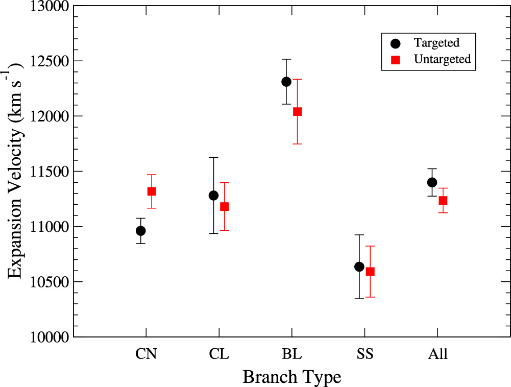
Figure 7. Average expansion velocities of the Si ii λ6355 for each of the Branch types in the targeted and untargeted samples, and for each of the two samples together. The error bars represent the standard errors of the mean.
Download figure:
Standard image High-resolution image4.4. Correlations between pW Values of Different Features at Maximum Light
In their study of SNe Ia from CSP-I, Folatelli et al. (2013) searched for correlations between the different pW measurements at maximum light. In Figures 8–11, we reproduce the four strongest correlations that they found, plotting each separately for the targeted and untargeted samples. Folatelli et al. found that the correlations were tighter (Pearson correlation coefficients ρ > ∣0.75∣) if the high-velocity and fast-declining (v(Si ii(6355) <12,000 km s−1 and Δm15(B) < 1.7 mag) events were excluded from the fits, but in this paper, we do not make this distinction. In each of Figures 8–11, coefficients of determination (R2) and Pearson correlation coefficients (r) are shown near the top-left or bottom-right corners of each panel.
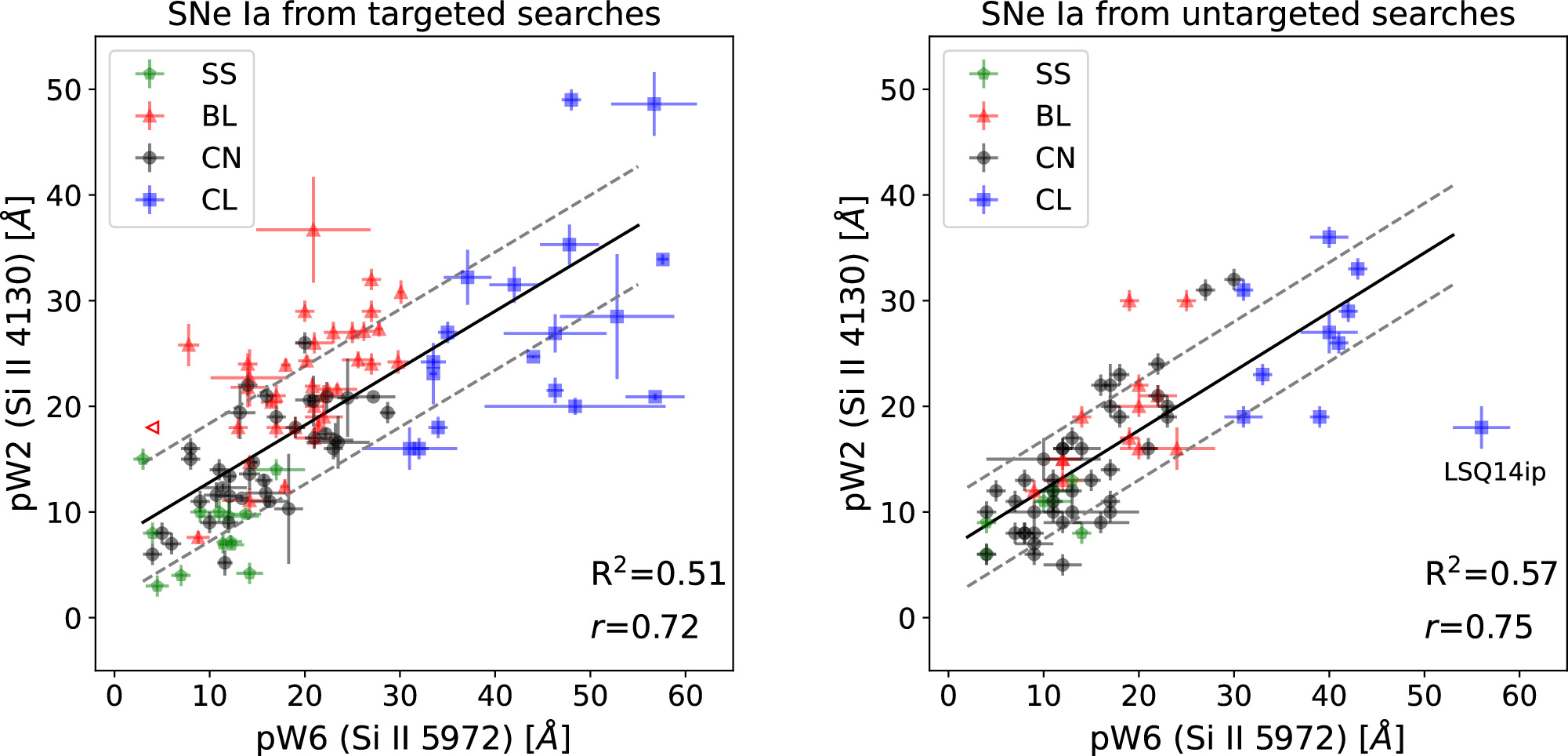
Figure 8. Correlation between pW values of Si ii λ4130 and Si ii λ5972 for our two different samples: historical SNe Ia and CSP SNe Ia from targeted searches (left) and CSP SNe Ia discovered by untargeted searches (right). The meaning of the symbols is as in Figure 4. The correlation strengths are similar for both samples, as well as the slopes of the best-fit lines (0.54 ± 0.05 and 0.56 ± 0.06 for the targeted and untargeted samples, respectively).
Download figure:
Standard image High-resolution imageAs shown in the right panel of Figure 8, the strongest correlation for the untargeted sample is found between the pW values for Si ii λ4130 versus Si ii λ5972. In this plot, the CL SN Ia LSQ14ip appears as an outlier in an otherwise strong positive correlation. However, the left panel of Figure 8 corresponding to the targeted sample shows a large dispersion in the measurements for the CL SNe Ia, with LSQ14ip lying within this dispersion. LSQ14ip is an extremely cool SN Ia, very similar to SN 1986G (Phillips et al. 1987), which showed strong Ti ii absorption at maximum light. The Si ii λ4130 line is blended with the Ti ii absorption (e.g., see Ashall et al. 2016), making it difficult to measure an accurate pW value. This blending undoubtedly accounts for the large dispersion in the CL events observed in the targeted sample.
In Figure 9, we plot the pW values for the Si ii λ4130 and Si ii λ6355 absorptions. In this case, the correlation is tighter for the targeted sample. As might be expected, however, correlations between all three of the Si ii lines are similarly strong for both the targeted and untargeted samples.
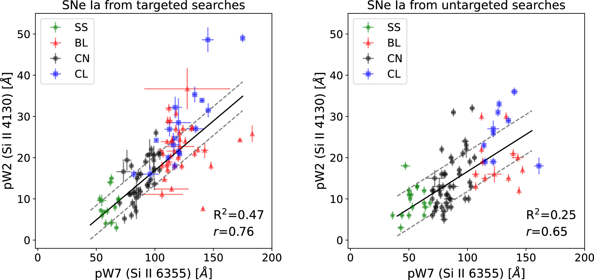
Figure 9. Correlation between pW values of Si ii λ4130 and Si ii λ6355 for our two different samples of SNe Ia discovered by targeted (left) and untargeted (right) searches. The meaning of the symbols is as in Figure 4. The correlation is stronger and has a smaller intrinsic scatter for the targeted sample. The best-fit lines have slopes of 0.24 ± 0.04 and 0.18 ± 0.04 for the targeted and untargeted samples, respectively.
Download figure:
Standard image High-resolution imageFigure 10 displays the pW values for the Ca ii IR triplet plotted versus the pW4 (Fe ii) measurements. The correlation is tighter for the SNe Ia discovered in untargeted searches. In Figure 11, the correlation between the pW8 (Ca ii IR) and pW7 (Si ii 6355) parameters is displayed. We see that the source of much of the dispersion, notably in the plot corresponding to the targeted searches, comes from the CL SNe Ia.
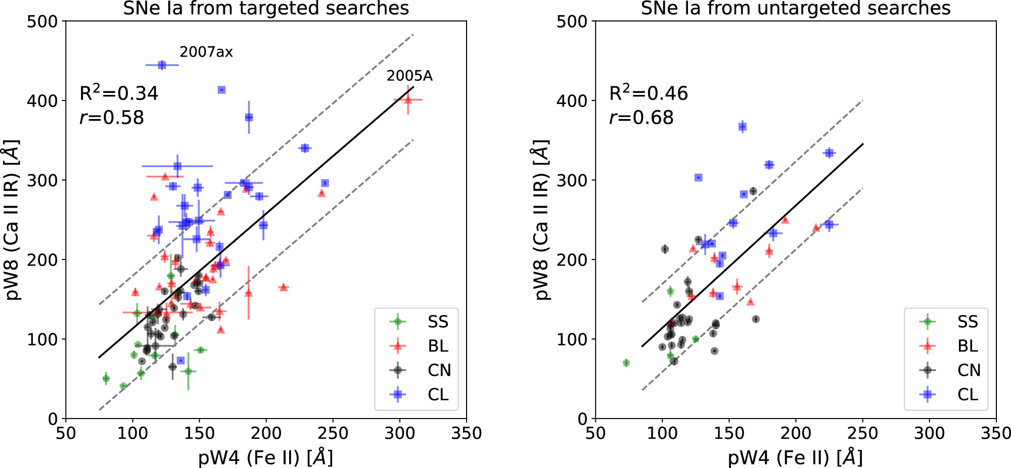
Figure 10. Correlation between pW values of the Ca ii IR triplet and the Fe ii feature at ∼4600 Å for our two different samples of SNe Ia discovered by targeted (left) and untargeted (right) searches. The meaning of the symbols is as in Figure 4. The correlation is a bit stronger for the untargeted sample, while the slopes are indistinguishable (1.51 ± 0.21 and 1.54 ± 0.24 for the targeted and untargeted samples, respectively).
Download figure:
Standard image High-resolution image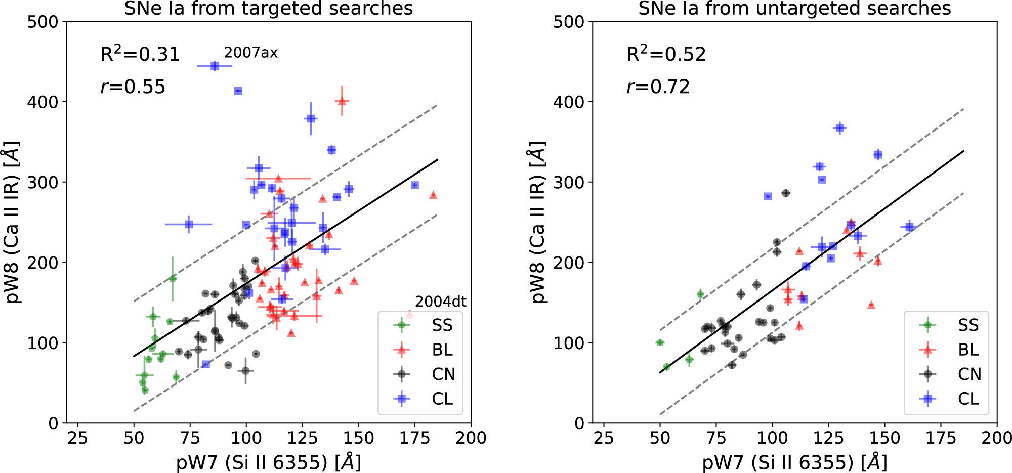
Figure 11. Correlation between pW values at maximum light of the Ca ii IR triplet and Si ii λ6355 for our two different samples of SNe Ia discovered by targeted (left) and untargeted (right) searches. The meaning of the symbols is as in Figure 4. The slopes of the best-fit lines are equivalent within the uncertainties: 1.81 ± 0.27 and 2.04 ± 0.28 for the targeted and untargeted samples, respectively.
Download figure:
Standard image High-resolution imageIn order to provide a broader view of the possible correlations between the spectroscopic parameters under consideration, in Figure 12, we present correlation matrices for pairs of pW values and expansion velocities at maximum light for the objects in our targeted and untargeted samples, respectively.
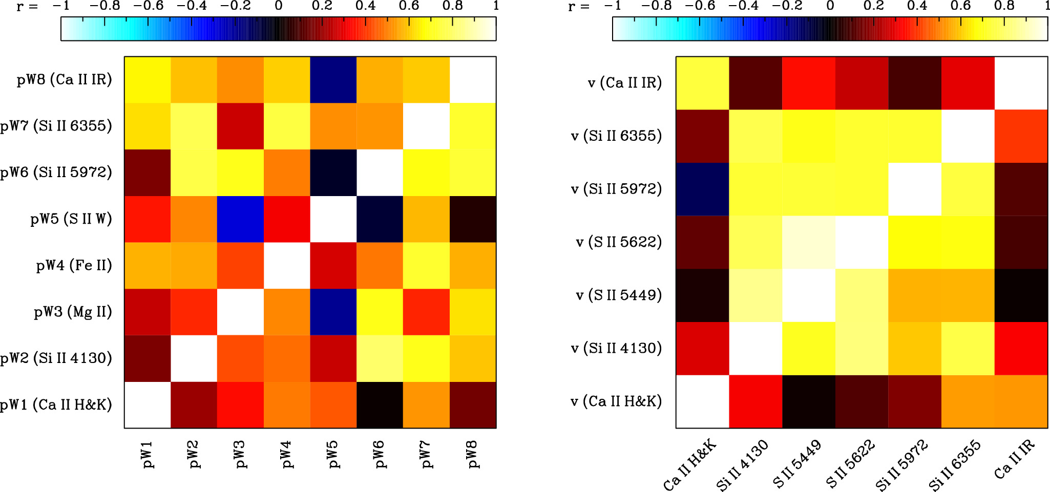
Figure 12. Correlation matrices for pairs of pWs (left) and expansion velocities (right) at maximum light for all the SNe Ia analyzed in this paper. The upper-left off-diagonal triangle of each matrix shows results for the targeted sample, while the lower right off-diagonal triangle represents the SNe Ia discovered in untargeted searches. As shown in the color scales on top of each panel, different colors correspond to different values of the Pearson coefficient (r), with lighter colors indicating stronger correlation (or anticorrelation).
Download figure:
Standard image High-resolution image4.5. Correlations Involving Spectroscopic Parameters at Maximum Light and Photometric Properties
Here, we briefly review the strongest correlations between pW values at maximum light and the light-curve decline rate expressed by the typical Δm15 parameter, or the more recently defined color stretch parameter, sBV. Figure 13 shows the correlations between pW6 (Si ii 5972) and Δm15. Hachinger et al. (2006) first pointed out that these two parameters correlate strongly. The relations are similarly tight for both the targeted and untargeted samples. The most discrepant measurements in the untargeted sample correspond to the CNs SN 2007ol and SN OGLE-2013-SN-123. As explained in Section 3.3, the PESSTO spectrum of the latter suffered from considerable host galaxy contamination. While our attempt to correct for this problem was largely successful, the error in the pW6 (Si ii 5972) measurement is likely underestimated due to uncertainties in the subtraction of the host galaxy spectrum. Accounting for this extra source of uncertainty would bring the error in pW6 up to ±7 Å. On the other hand, the spectrum of SN 2007ol looks good and does not show indications of host galaxy contamination.
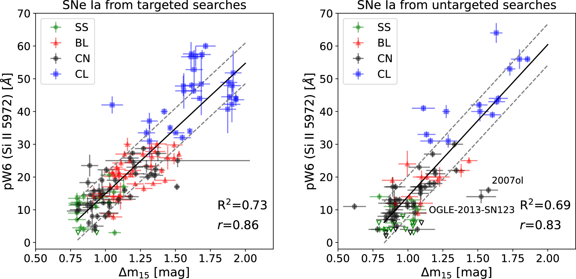
Figure 13. pW at maximum light of Si ii λ5972 vs. Δm15 for our two different samples of SNe Ia discovered by targeted (left) and untargeted (right) searches. The meaning of the symbols is as in Figure 4. The best-fit lines have slopes of 39.8 ± 2.2 Å per mag, and 46.4 ± 3.5 Å per mag for the targeted and untargeted samples, respectively.
Download figure:
Standard image High-resolution imageFigure 14 displays the relationship between pW6 (Si ii 5972) and sBV. We might have expected an improvement in the correlation since the sBV parameter does a better job of discriminating between light-curve shapes for fast-declining events. Nevertheless, the coefficients of determination and Pearson r coefficients are similar to those obtained using Δm15.
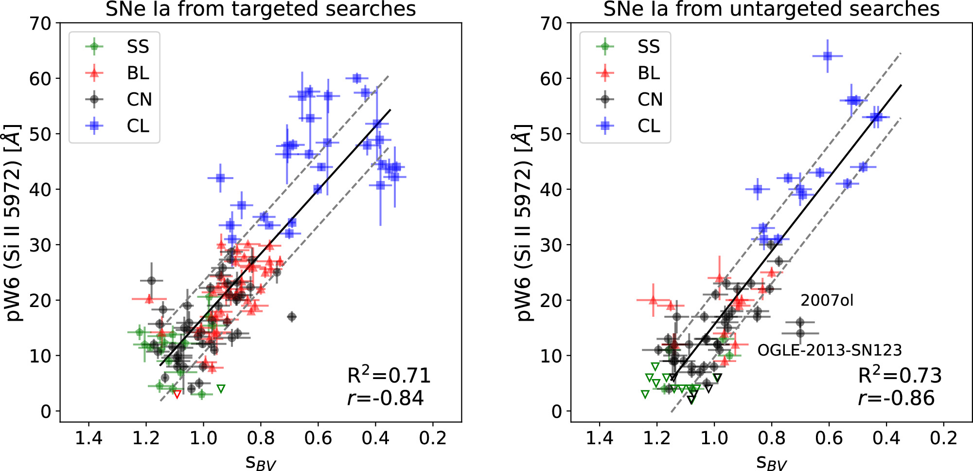
Figure 14. pW at maximum light of Si ii λ5972 vs. color stretch for our two different samples of SNe Ia discovered by targeted (left) and untargeted (right) searches. The meaning of the symbols is as in Figure 4. The slopes of the best-fit lines are −57.4 Å ± 3.2 Å and −66.4 Å ± 4.4 Å for the targeted and untargeted samples, respectively. In this figure, the abscissa has been inverted to facilitate comparison with Figure 13.
Download figure:
Standard image High-resolution imageFolatelli et al. (2013) found that pW2 (Si ii 4130) also correlated strongly with the light-curve decline rate. In Figures 15 and 16, this parameter is plotted against Δm15 and sBV, respectively. Again, it is somewhat surprising to see that usage of sBV does not significantly improve the tightness of the correlations. This could be related to the fact that sBV seems not to work as well as Δm15 for SS SNe Ia (C. Burns, private communication).

Figure 15. pW at maximum light of Si ii λ4130 vs. Δm15 for our two different samples of SNe Ia discovered by targeted (left) and untargeted (right) searches. The meaning of the symbols is as in Figure 4. The slopes of the best-fit lines are 25.2 ± 2.6 Å per mag, and 26.1 ± 3.1 Å per mag, for the targeted and untargeted samples, respectively.
Download figure:
Standard image High-resolution image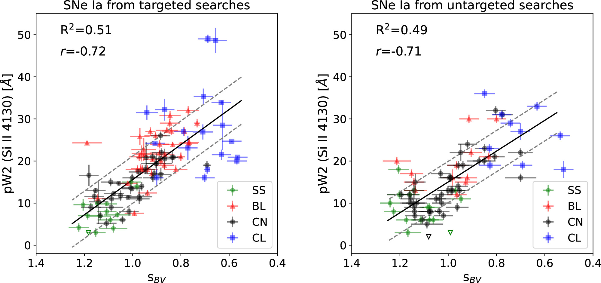
Figure 16. pW at maximum light of Si ii λ4130 vs. color stretch for our two different samples of SNe Ia discovered by targeted (left) and untargeted (right) searches. The meaning of the symbols is as in Figure 4. The slopes of the best-fit lines are −41.7 Å ± 4.1 Å and 36.6 Å ± 4.0 Å for the targeted and untargeted samples, respectively. Note that the abscissa (sBV) is inverted in this plot to facilitate comparison with Figure 15.
Download figure:
Standard image High-resolution image
5. Summary
In this paper, we have presented 230 optical spectra of 130 SNe Ia observed during the course of the CSP-II campaign, which was carried out between 2011 and 2015. These data are complemented by an additional 148 optical spectra of 30 SNe Ia obtained during the CSP-I campaign (2004–2009) that were not included in the paper by Folatelli et al. (2013). Finally, we have appended to this paper a historical sample consisting of 53 spectra of 30 SNe Ia observed by the Calán/Tololo Supernova Survey between 1990 and 1993, along with 163 additional spectra of 16 SNe Ia obtained between 1986 and 2001, mostly by members of the Calán/Tololo team. A number of optical spectra of SNe Ia obtained in the course of the CSP campaigns already published in previous papers have also been considered in this work. Measurements of expansion velocities at maximum light, the Si ii λ6355 velocity decline parameter, Δv20(Si ii), and pW features at maximum light in the system of Garavini et al. (2007) and Folatelli et al. (2013) have been provided for as many of these SNe Ia as possible. These data have been combined with measurements of the same parameters for the CSP-I SNe Ia published by Folatelli et al. (2013) to reexamine the Branch diagram and a few of the strongest correlations of parameters found for SNe Ia discovered in targeted versus untargeted searches. The most significant difference that we find is in the Branch diagram for targeted searches, which contains proportionately more CL and BL objects than is the case for untargeted searches. This difference is ascribed to the fact that targeted searches are dominated by SNe Ia discovered in luminous galaxies, and that CL and BL events are known to preferentially occur in such galaxies.
Acknowledgments
The work of the CSP has been supported by the National Science Foundation under grants AST0306969, AST0607438, AST1008343, AST1613426, AST1613455, and AST1613472. CSP-II was also supported in part by funding from the Danish Villum FONDEN (grant Nos. 13261 and 28021) and the Independent Research Fund Denmark (IRFD) by a Sapere Aude II Fellowship awarded to M.D.S. Additional IRFD funding comes from Project 1 (8021-00170B) and Project 2 (10.46540/2032-00022B) grants. This paper includes data gathered with the 6.5 m Magellan Telescopes located at Las Campanas Observatory, the Gemini South, Cerro Pachón, Chile, and Gemini North, Maunakea, Hawaii (Gemini Program Nos. GS-2011B-Q-15-150-002 and GN-2013A-Q-68-82-002). Also based on observations collected at the European Organization for Astronomical Research in the Southern Hemisphere, Chile (ESO Programs 164.H-0376 and 0102.D-0095). C.G. is supported by a research grant (25501) by the Villum FONDEN. M.H. acknowledges support from FONDECYT-Chile through grants 92/0312 and 1060808; the National Science Foundation through grants GF-1002-96 and GF-1002-97; the Association of Universities for Research in Astronomy, Inc., under NSF Cooperative Agreement AST-8947990 and from Fundación Andes under project C-12984; the Hubble Fellowship grant HST-HF-01139.01-A (awarded by the Space Telescope Science Institute, which is operated by the Association of Universities for Research in Astronomy, Inc., for NASA, under contract NAS 5-26555); and the Carnegie Postdoctoral Fellowship. This work has been funded by ANID, Millennium Science Initiative, ICN12_009. L.G. acknowledges financial support from the Spanish Ministerio de Ciencia e Innovación (MCIN), the Agencia Estatal de Investigación (AEI) 10.13039/501100011033, and the European Social Fund (ESF) "Investing in your future" under the 2019 Ramón y Cajal program RYC2019-027683-I and the PID2020-115253GA-I00 HOSTFLOWS project, from Centro Superior de Investigaciones Científicas (CSIC) under the PIE project 20215AT016, and the program Unidad de Excelencia María de Maeztu CEX2020-001058-M. C.A. acknowledges support by NASA grants JWST-GO-02114, JWST-GO-02122, and JWST-GO-04436.024-A; and JPL grant SS03-17-23. The research of J.C.W. and J.V. is supported by NSF AST-1813825. J.V. is also supported by OTKA grant K-142534 of the National Research, Development and Innovation Office, Hungary. The authors want to thank an anonymous referee for their kind report and useful suggestions.
Facilities: Magellan:Baade (IMACS imaging spectrograph) - , Magellan:Clay - Magellan II Landon Clay Telescope (LDSS3, MagE, MIKE), Du Pont (WFCCD, B&C spectrograph, MODSPEC), ESO 3.6 m (EFOSC-2), NTT (EMMI), ESO 1.52 m (B&C spectrograph), VLT:Yepun (MUSE), NOT (ALFOSC), Gemini:South (GMOS), Gemini:Gillett (GMOS), CTIO 1.0 m (B&C spectrograph), CTIO 1.5 m (R-C spectrograph), Blanco (R-C spectrograph), UH 2.2 m, KPNO 2.1 m (Gold camera), MMT (red channel), Shane (Cassegrain spectrograph), Nickel (Cassegrain spectrograph), FLWO 1.5 m (Z- Machine), ESO:Schmidt (QUEST camera), SO:Schmidt, Uppsala Schmidt, SO:1.5m, PO:1.2m, OGLE, ASAS-SN, PS1, Kiso:Schmidt, ISSP, MASTER, Skymapper, CTIO:Schmidt, CTIO:0.9m.
Footnotes
- 44
The redshift quoted here is not precisely the redshift as defined in cosmology, in that it can contain peculiar velocities due to galaxy infall. If an averaged peculiar velocity of 300 km s−1 is assumed, it would add a 0.001 uncertainty in the redshift, as estimated from the spectroscopic velocity.
- 45
Δm15 is approximately equivalent to Δm15(B), but is measured via SNooPy fits to all photometric filters available, rather than being a direct measurement of the B-band light-curve decline rate.
- 46
IRAF was distributed by the National Optical Astronomy Observatory, which is operated by the Association of Universities for Research in Astronomy, Inc., under cooperative agreement with the National Science Foundation.
- 47
Public ESO Spectroscopic Survey of Transient Objects, Smartt et al. (2015).
- 48
All the correlations presented in this work have been computed via the linmix code (https://github.com/jmeyers314/linmix) based on Kelly (2007). In the corresponding figures we present the data along with best-fit lines, intrinsic scatter lines, coefficients of determination (R2) and Pearson correlation coefficients (r).